PyTorch CNN

深度学习系列：第 1 篇，共 22 篇

用 PyTorch 从搭建模型、训练、调试到部署的一组笔记。按下面的顺序阅读，后面的文章会直接引用前面讲过的内容

模型结构

1. PyTorch CNN
2. PyTorch Transformer
3. Vision Transformer

训练

4. PyTorch Data Loading
5. PyTorch Training
6. Optimizers and Learning Rate Schedules
7. PyTorch Checkpoints and Reproducibility
8. Normalization and Regularization
9. PyTorch Debugging
10. PyTorch Common Mistakes
11. PyTorch Memory and Speed
12. Evaluation Metrics
13. TensorBoard
14. Experiment Tracking
15. PyTorch Distributed Training

任务

16. PyTorch Fine-Tuning
17. Object Detection
18. Image Segmentation
19. Keypoint Detection
20. Generative Models

部署

21. PyTorch Deployment
22. Model Compression

卷积神经网络（CNN）由卷积、池化等层堆叠而成。PyTorch 中二维图像张量的形状为$(N, C, H, W)$，依次为批大小、通道数、高度和宽度。卷积、池化等层只改变$C$、$H$、$W$，不改变$N$

输出尺寸计算

通用公式

kernel_size、stride、padding、dilation可以是一个整数（高度和宽度方向相同），也可以是(高度, 宽度)形式的元组。高度和宽度是分别独立计算的，使用同一个公式，下面只写其中一个方向，把该方向的输入长度记作$L$

符号	对应参数	含义
$K$	kernel_size	卷积核或池化窗口的大小
$S$	stride	步幅，每次移动的距离
$P$	padding	填充，在两侧各补多少
$D$	dilation	膨胀，核内相邻两个元素的间距，默认为 1
$O$	output_padding	转置卷积在输出一侧额外增加的长度

膨胀会让卷积核在输入上覆盖更大的范围，覆盖的实际长度称为等效核大小，记作$K’$，不使用膨胀时$K’ = K$

\[K' = D \cdot (K - 1) + 1\]

卷积和池化的输出长度为

\[L_{out} = \left\lfloor \frac{L + 2P - K'}{S} \right\rfloor + 1\]

填充后的总长度为$L + 2P$，放下第一个核之后还剩$L + 2P - K’$，每移动$S$就多出一个输出，移动到放不下为止，所以向下取整

以$5 \times 5$的输入、kernel_size=3、stride=2、padding=1为例，卷积核每次移动 2 格，在每个方向上可以放置 3 个位置，输出为$3 \times 3$

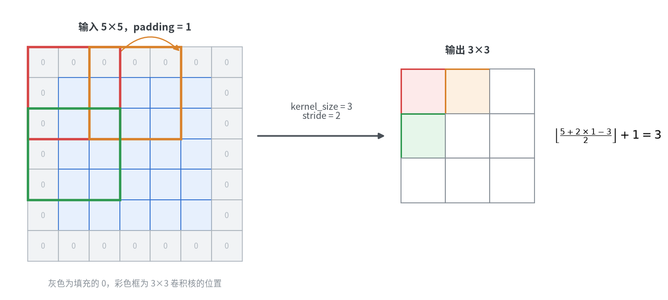
一维的nn.Conv1d和三维的nn.Conv3d同样适用这个公式，只是需要计算的方向数不同

各层的输出尺寸

层	高度和宽度	通道数
nn.Conv2d	按通用公式	变为out_channels
nn.MaxPool2d	按通用公式，stride默认等于kernel_size	不变
nn.AvgPool2d	按通用公式，没有dilation参数	不变
nn.ConvTranspose2d	按转置卷积的公式，见下文	变为out_channels
nn.AdaptiveAvgPool2d nn.AdaptiveMaxPool2d	等于指定的output_size	不变
nn.Upsample	乘以scale_factor，或等于指定的size	不变
nn.PixelShuffle	乘以upscale_factor	除以upscale_factor的平方
nn.BatchNorm2d、nn.ReLU、nn.Dropout	不变	不变
nn.Flatten	与通道合并为一维	变为$C \times H \times W$

卷积层

nn.Conv2d(in_channels, out_channels, kernel_size, stride=1, padding=0, dilation=1, groups=1, bias=True)

常用的几种组合：

kernel_size	stride	padding	输出大小
3	1	1	与输入相同
5	1	2	与输入相同
3	2	1	输入的一半（向上取整）
1	1	0	与输入相同，只改变通道数

padding也可以写成字符串：'same'自动计算使输出与输入大小相同的填充（仅支持stride=1），'valid'表示不填充

import torch
from torch import nn

x = torch.randn(1, 3, 224, 224)

print(nn.Conv2d(3, 16, kernel_size=3, stride=1, padding=1)(x).shape)  # torch.Size([1, 16, 224, 224])
print(nn.Conv2d(3, 16, kernel_size=3, stride=2, padding=1)(x).shape)  # torch.Size([1, 16, 112, 112])
print(nn.Conv2d(3, 16, kernel_size=3, dilation=2)(x).shape)           # torch.Size([1, 16, 220, 220])
print(nn.Conv2d(3, 16, kernel_size=(3, 5), padding=(1, 2))(x).shape)  # torch.Size([1, 16, 224, 224])
print(nn.Conv2d(3, 16, kernel_size=3, padding='same')(x).shape)       # torch.Size([1, 16, 224, 224])

池化层

nn.MaxPool2d(kernel_size, stride=None, padding=0, dilation=1, ceil_mode=False)
nn.AvgPool2d(kernel_size, stride=None, padding=0, ceil_mode=False)
nn.AdaptiveAvgPool2d(output_size)
nn.AdaptiveMaxPool2d(output_size)

• stride默认为None，表示与kernel_size相同，因此nn.MaxPool2d(2)会使高度和宽度减半
• ceil_mode设为True时，通用公式中的向下取整改为向上取整，输入长度不能被整除时会多出一个输出
• 自适应池化直接指定输出大小，由 PyTorch 自动确定窗口和步幅。nn.AdaptiveAvgPool2d(1)即全局平均池化，常用于分类网络中全连接层之前，使网络可以接受任意大小的输入

import torch
from torch import nn

x = torch.randn(1, 16, 7, 7)

print(nn.MaxPool2d(kernel_size=2)(x).shape)                  # torch.Size([1, 16, 3, 3])
print(nn.MaxPool2d(kernel_size=2, ceil_mode=True)(x).shape)  # torch.Size([1, 16, 4, 4])
print(nn.AvgPool2d(kernel_size=3, stride=2, padding=1)(x).shape)  # torch.Size([1, 16, 4, 4])
print(nn.AdaptiveAvgPool2d(1)(x).shape)                      # torch.Size([1, 16, 1, 1])
print(nn.AdaptiveMaxPool2d((2, 3))(x).shape)                 # torch.Size([1, 16, 2, 3])

转置卷积层

nn.ConvTranspose2d(in_channels, out_channels, kernel_size, stride=1, padding=0, output_padding=0, dilation=1)

转置卷积用于上采样，输出长度的计算与卷积相反

\[L_{out} = (L - 1) \cdot S - 2P + K' + O\]

卷积在步幅大于 1 时向下取整，多个不同的输入长度会得到相同的输出长度，例如 223 和 224 经过kernel_size=3、stride=2、padding=1的卷积都得到 112。反过来做转置卷积时，output_padding用于指定还原到其中的哪一个

其他上采样方式

• nn.Upsample通过插值放大特征图，没有需要学习的参数
• nn.PixelShuffle把通道重新排列到空间上，通道数除以放大倍数的平方，常用于超分辨率

import torch
from torch import nn

conv = nn.Conv2d(3, 16, kernel_size=3, stride=2, padding=1)
print(conv(torch.randn(1, 3, 223, 223)).shape)  # torch.Size([1, 16, 112, 112])
print(conv(torch.randn(1, 3, 224, 224)).shape)  # torch.Size([1, 16, 112, 112])

y = torch.randn(1, 16, 112, 112)
print(nn.ConvTranspose2d(16, 3, kernel_size=3, stride=2, padding=1)(y).shape)                    # torch.Size([1, 3, 223, 223])
print(nn.ConvTranspose2d(16, 3, kernel_size=3, stride=2, padding=1, output_padding=1)(y).shape)  # torch.Size([1, 3, 224, 224])

print(nn.Upsample(scale_factor=2)(y).shape)  # torch.Size([1, 16, 224, 224])
print(nn.PixelShuffle(2)(y).shape)           # torch.Size([1, 4, 224, 224])

全连接层的输入维度

计算输出尺寸最常见的用途，是确定卷积部分之后第一个nn.Linear的in_features。nn.Flatten把$(N, C, H, W)$展平为$(N, C \times H \times W)$，全连接层的输入维度就是最后一个特征图的$C \times H \times W$

以输入为$3 \times 32 \times 32$的小型分类网络为例，逐层推导如下

层	计算	输出形状
Conv2d(3, 16, 3, padding=1)	(32 + 2×1 − 3) / 1 + 1 = 32	16 × 32 × 32
MaxPool2d(2)	(32 − 2) / 2 + 1 = 16	16 × 16 × 16
Conv2d(16, 32, 3, padding=1)	(16 + 2×1 − 3) / 1 + 1 = 16	32 × 16 × 16
MaxPool2d(2)	(16 − 2) / 2 + 1 = 8	32 × 8 × 8
Flatten()	32 × 8 × 8	2048
Linear(2048, 10)		10

import torch
from torch import nn

model = nn.Sequential(
    nn.Conv2d(3, 16, kernel_size=3, padding=1),
    nn.ReLU(),
    nn.MaxPool2d(2),
    nn.Conv2d(16, 32, kernel_size=3, padding=1),
    nn.ReLU(),
    nn.MaxPool2d(2),
    nn.Flatten(),
    nn.Linear(32 * 8 * 8, 10),
)

x = torch.randn(1, 3, 32, 32)
print(model(x).shape)  # torch.Size([1, 10])

不想手动计算时，可以使用nn.LazyLinear，它的in_features在第一次前向传播时根据输入自动确定。nn.LazyConv2d等同理

import torch
from torch import nn

model = nn.Sequential(
    nn.Conv2d(3, 16, kernel_size=3, padding=1),
    nn.ReLU(),
    nn.MaxPool2d(2),
    nn.Flatten(),
    nn.LazyLinear(10),  # in_features在第一次前向传播时自动确定
)

model(torch.randn(1, 3, 32, 32))
print(model[-1].in_features)  # 4096

参数量计算

参数量只与层自身的配置有关，与输入的高度和宽度无关

层	参数量	说明
nn.Conv2d	（核高 × 核宽 × 输入通道数 ÷ groups + 1）× 输出通道数	括号中的 1 为偏置，bias=False时去掉
nn.Linear	（输入维度 + 1）× 输出维度	同上
nn.BatchNorm2d	2 × 通道数	每个通道一个缩放系数和一个偏移
池化、激活、nn.Flatten、nn.Upsample	0	没有需要学习的参数

groups把输入通道分成若干组，各组分别卷积。groups等于输入通道数时每个通道单独卷积，称为逐通道卷积；后面再接一个$1 \times 1$卷积混合各通道，就是深度可分离卷积，参数量远小于普通卷积

from torch import nn


def count(module):
    return sum(p.numel() for p in module.parameters())


print(count(nn.Conv2d(3, 16, kernel_size=3)))              # 448
print(count(nn.Conv2d(3, 16, kernel_size=3, bias=False)))  # 432
print(count(nn.Linear(2048, 10)))                          # 20490
print(count(nn.BatchNorm2d(16)))                           # 32

# 普通卷积与深度可分离卷积
standard = nn.Conv2d(32, 64, kernel_size=3, padding=1)
separable = nn.Sequential(
    nn.Conv2d(32, 32, kernel_size=3, padding=1, groups=32),  # 逐通道卷积
    nn.Conv2d(32, 64, kernel_size=1),                        # 逐点卷积
)
print(count(standard))   # 18496
print(count(separable))  # 2432

感受野计算

感受野是输出特征图上的一个点对应到输入图像上的区域大小。感受野越大，这个点能”看到”的上下文越多；要识别的目标比感受野大时，网络无法看到完整的目标

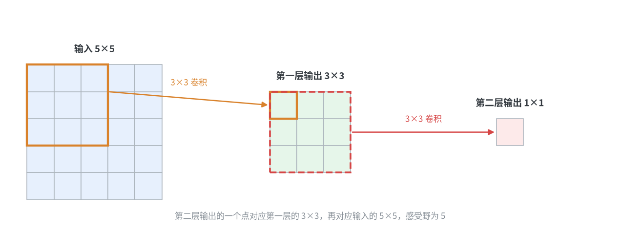
从输入开始逐层递推，同时记录两个量：感受野$r$和间隔$j$（输出上相邻两个点对应到输入上相隔多少个像素）。初始值都为 1，每经过一层

\[r_{l} = r_{l-1} + (K'_{l} - 1) \cdot j_{l-1} ,\qquad j_{l} = j_{l-1} \cdot S_{l}\]

• 卷积核越大、层数越多，感受野越大
• 步幅会放大之后所有层对感受野的贡献，因此下采样之后感受野增长得更快
• 膨胀卷积通过增大等效核大小来扩大感受野，不增加参数量
• 填充不影响感受野的大小

def receptive_field(layers):
    """layers: 由(kernel_size, stride, dilation)组成的列表，按前向顺序排列"""
    size, jump = 1, 1
    for kernel_size, stride, dilation in layers:
        effective = dilation * (kernel_size - 1) + 1
        size += (effective - 1) * jump
        jump *= stride
    return size


print(receptive_field([(3, 1, 1), (2, 2, 1), (3, 1, 1), (2, 2, 1)]))  # 10，上文的小型分类网络
print(receptive_field([(3, 1, 1)] * 2))                               # 5，两个3x3相当于一个5x5
print(receptive_field([(3, 1, 1)] * 3))                               # 7，三个3x3相当于一个7x7
print(receptive_field([(3, 1, 1), (3, 1, 2), (3, 1, 4)]))             # 15，膨胀卷积

多个小卷积核堆叠可以得到与大卷积核相同的感受野，而参数更少：两个$3 \times 3$卷积的参数量是一个$5 \times 5$卷积的 18/25，中间还多一次非线性变换，这也是现在的网络普遍使用$3 \times 3$卷积的原因

公式给出的是理论感受野，可以用梯度验证：只对输出中的一个点反向传播，输入上梯度不为零的范围就是它的感受野

import torch
from torch import nn

model = nn.Sequential(
    nn.Conv2d(1, 1, kernel_size=3, padding=1),
    nn.AvgPool2d(2),
    nn.Conv2d(1, 1, kernel_size=3, padding=1),
    nn.AvgPool2d(2),
)

x = torch.randn(1, 1, 64, 64, requires_grad=True)
y = model(x)
y[0, 0, 8, 8].backward()  # 只对输出中间的一个点求梯度

rows = x.grad[0, 0].abs().sum(dim=1).nonzero().flatten()
print(int(rows.max() - rows.min() + 1))  # 10，该输出点最多受输入中10行的影响

验证时用的是平均池化。最大值池化只把梯度传给窗口内最大的那个位置，实测到的范围会小于理论值

常用结构

实际的网络很少直接堆叠单个卷积层，而是由一些固定的结构重复组合而成

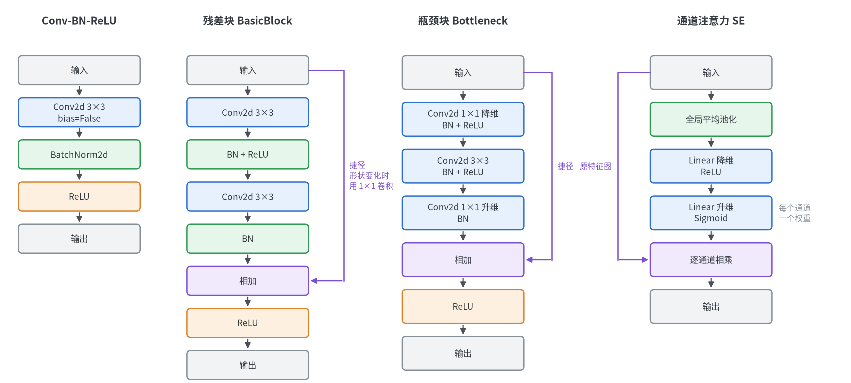
结构	作用	常见于
Conv-BN-ReLU	最基本的卷积单元	几乎所有卷积网络
残差块	通过捷径把输入加到输出上，使很深的网络也能训练	ResNet-18、ResNet-34
瓶颈块	先降维再卷积再升维，减少深层网络的计算量	ResNet-50 及更深的 ResNet
深度可分离卷积	用逐通道卷积加逐点卷积代替普通卷积，大幅减少参数	MobileNet 等轻量网络
通道注意力	为每个通道学习一个权重，突出有用的通道	SENet，也可插入其他网络
上采样拼接	放大深层特征并与浅层特征拼接，恢复细节	U-Net 等分割网络
分类头	把特征图变为类别得分	各类分类网络

以下代码按顺序放在同一个文件中，后面的结构会用到前面的导入和ConvBNReLU

Conv-BN-ReLU

卷积、批归一化、激活函数依次连接。卷积后面紧跟BatchNorm2d时，卷积的偏置会被归一化抵消，因此设置bias=False；padding=kernel_size // 2使步幅为 1 时输出大小不变

import torch
from torch import nn


class ConvBNReLU(nn.Sequential):
    def __init__(self, in_channels, out_channels, kernel_size=3, stride=1):
        super().__init__(
            nn.Conv2d(in_channels, out_channels, kernel_size, stride,
                      padding=kernel_size // 2, bias=False),
            nn.BatchNorm2d(out_channels),
            nn.ReLU(inplace=True),
        )


x = torch.randn(1, 3, 224, 224)
print(ConvBNReLU(3, 32)(x).shape)            # torch.Size([1, 32, 224, 224])
print(ConvBNReLU(3, 32, stride=2)(x).shape)  # torch.Size([1, 32, 112, 112])

残差块

两个$3 \times 3$卷积，加上一条把输入直接加到输出上的捷径。相加要求两边形状相同，步幅不为 1 或通道数改变时，捷径上用一个$1 \times 1$卷积把输入调整到相同的形状

class BasicBlock(nn.Module):
    def __init__(self, in_channels, out_channels, stride=1):
        super().__init__()
        self.conv1 = nn.Conv2d(in_channels, out_channels, 3, stride, padding=1, bias=False)
        self.bn1 = nn.BatchNorm2d(out_channels)
        self.conv2 = nn.Conv2d(out_channels, out_channels, 3, padding=1, bias=False)
        self.bn2 = nn.BatchNorm2d(out_channels)
        self.relu = nn.ReLU(inplace=True)

        # 形状发生变化时，捷径分支用1x1卷积把输入调整到相同的形状
        self.shortcut = nn.Identity()
        if stride != 1 or in_channels != out_channels:
            self.shortcut = nn.Sequential(
                nn.Conv2d(in_channels, out_channels, 1, stride, bias=False),
                nn.BatchNorm2d(out_channels),
            )

    def forward(self, x):
        out = self.relu(self.bn1(self.conv1(x)))
        out = self.bn2(self.conv2(out))
        return self.relu(out + self.shortcut(x))


x = torch.randn(1, 64, 56, 56)
print(BasicBlock(64, 64)(x).shape)             # torch.Size([1, 64, 56, 56])
print(BasicBlock(64, 128, stride=2)(x).shape)  # torch.Size([1, 128, 28, 28])

瓶颈块

通道数很大时，直接做$3 \times 3$卷积的计算量很大。瓶颈块先用$1 \times 1$卷积把通道数降到四分之一，在较少的通道上做$3 \times 3$卷积，再用$1 \times 1$卷积升回去。同样是 256 个通道，瓶颈块的参数量约 7 万，由两个$3 \times 3$卷积组成的残差块约 118 万

class Bottleneck(nn.Module):
    expansion = 4

    def __init__(self, in_channels, mid_channels, stride=1):
        super().__init__()
        out_channels = mid_channels * self.expansion
        self.body = nn.Sequential(
            nn.Conv2d(in_channels, mid_channels, 1, bias=False),  # 1x1降维
            nn.BatchNorm2d(mid_channels),
            nn.ReLU(inplace=True),
            nn.Conv2d(mid_channels, mid_channels, 3, stride, padding=1, bias=False),
            nn.BatchNorm2d(mid_channels),
            nn.ReLU(inplace=True),
            nn.Conv2d(mid_channels, out_channels, 1, bias=False),  # 1x1升维
            nn.BatchNorm2d(out_channels),
        )
        self.relu = nn.ReLU(inplace=True)

        self.shortcut = nn.Identity()
        if stride != 1 or in_channels != out_channels:
            self.shortcut = nn.Sequential(
                nn.Conv2d(in_channels, out_channels, 1, stride, bias=False),
                nn.BatchNorm2d(out_channels),
            )

    def forward(self, x):
        return self.relu(self.body(x) + self.shortcut(x))


x = torch.randn(1, 256, 56, 56)
print(Bottleneck(256, 64)(x).shape)             # torch.Size([1, 256, 56, 56])
print(Bottleneck(256, 128, stride=2)(x).shape)  # torch.Size([1, 512, 28, 28])

深度可分离卷积

把普通卷积拆成两步：逐通道卷积只在各通道内部提取空间特征，逐点卷积再混合各通道。32 通道到 64 通道时参数量为 2528，同样配置的普通卷积块为 18560

class DepthwiseSeparable(nn.Sequential):
    def __init__(self, in_channels, out_channels, stride=1):
        super().__init__(
            # 逐通道卷积：groups等于通道数，每个通道单独做3x3卷积
            nn.Conv2d(in_channels, in_channels, 3, stride, padding=1,
                      groups=in_channels, bias=False),
            nn.BatchNorm2d(in_channels),
            nn.ReLU(inplace=True),
            # 逐点卷积：1x1卷积混合各通道并改变通道数
            nn.Conv2d(in_channels, out_channels, 1, bias=False),
            nn.BatchNorm2d(out_channels),
            nn.ReLU(inplace=True),
        )


x = torch.randn(1, 32, 112, 112)
print(DepthwiseSeparable(32, 64)(x).shape)            # torch.Size([1, 64, 112, 112])
print(DepthwiseSeparable(32, 64, stride=2)(x).shape)  # torch.Size([1, 64, 56, 56])

通道注意力

先用全局平均池化把每个通道压缩成一个数，经过两层全连接得到每个通道的权重，再乘回原特征图。输出形状与输入相同，可以直接插入到其他结构中，增加的参数很少

class SEBlock(nn.Module):
    def __init__(self, channels, reduction=16):
        super().__init__()
        self.pool = nn.AdaptiveAvgPool2d(1)
        self.fc = nn.Sequential(
            nn.Linear(channels, channels // reduction),
            nn.ReLU(inplace=True),
            nn.Linear(channels // reduction, channels),
            nn.Sigmoid(),
        )

    def forward(self, x):
        n, c, _, _ = x.shape
        weight = self.fc(self.pool(x).view(n, c)).view(n, c, 1, 1)  # 每个通道一个0到1之间的权重
        return x * weight


x = torch.randn(1, 64, 56, 56)
print(SEBlock(64)(x).shape)  # torch.Size([1, 64, 56, 56])

上采样拼接

分割等任务需要把特征图恢复到输入的分辨率。深层特征分辨率低但语义强，浅层特征分辨率高但语义弱，把深层特征放大后与同分辨率的浅层特征在通道维度上拼接，再用卷积融合

class UpBlock(nn.Module):
    def __init__(self, in_channels, skip_channels, out_channels):
        super().__init__()
        self.up = nn.ConvTranspose2d(in_channels, in_channels // 2, kernel_size=2, stride=2)
        self.conv = ConvBNReLU(in_channels // 2 + skip_channels, out_channels)

    def forward(self, x, skip):
        x = self.up(x)                   # 高度和宽度放大2倍
        x = torch.cat([x, skip], dim=1)  # 在通道维度上拼接，要求高度和宽度相同
        return self.conv(x)


x = torch.randn(1, 128, 28, 28)    # 深层特征
skip = torch.randn(1, 64, 56, 56)  # 编码器中同分辨率的浅层特征
print(UpBlock(128, 64, 64)(x, skip).shape)  # torch.Size([1, 64, 56, 56])

分类头

全局平均池化把任意大小的特征图压缩为每个通道一个数，再接全连接层输出各类别的得分。由于池化后的大小固定，网络可以接受不同大小的输入

head = nn.Sequential(
    nn.AdaptiveAvgPool2d(1),  # (N, C, H, W) -> (N, C, 1, 1)
    nn.Flatten(),             # (N, C, 1, 1) -> (N, C)
    nn.Linear(512, 10),
)

print(head(torch.randn(1, 512, 7, 7)).shape)    # torch.Size([1, 10])
print(head(torch.randn(1, 512, 13, 9)).shape)   # torch.Size([1, 10])

查看各层的输出形状

实际搭建网络时，最直接的方法是构造一个与输入形状相同的张量，让它依次通过每一层并打印形状。以上面的小型分类网络model为例

x = torch.randn(1, 3, 32, 32)
for layer in model:
    x = layer(x)
    print(f"{layer.__class__.__name__:<10} {tuple(x.shape)}")

Conv2d     (1, 16, 32, 32)
ReLU       (1, 16, 32, 32)
MaxPool2d  (1, 16, 16, 16)
Conv2d     (1, 32, 16, 16)
ReLU       (1, 32, 16, 16)
MaxPool2d  (1, 32, 8, 8)
Flatten    (1, 2048)
Linear     (1, 10)

这种写法只适用于nn.Sequential。结构更复杂的网络可以使用torchinfo，它会同时列出每一层的输出形状和参数量

pip install torchinfo

from torchinfo import summary

summary(model, input_size=(1, 3, 32, 32))

==========================================================================================
Layer (type:depth-idx)                   Output Shape              Param #
==========================================================================================
Sequential                               [1, 10]                   --
├─Conv2d: 1-1                            [1, 16, 32, 32]           448
├─ReLU: 1-2                              [1, 16, 32, 32]           --
├─MaxPool2d: 1-3                         [1, 16, 16, 16]           --
├─Conv2d: 1-4                            [1, 32, 16, 16]           4,640
├─ReLU: 1-5                              [1, 32, 16, 16]           --
├─MaxPool2d: 1-6                         [1, 32, 8, 8]             --
├─Flatten: 1-7                           [1, 2048]                 --
├─Linear: 1-8                            [1, 10]                   20,490
==========================================================================================
Total params: 25,578
Trainable params: 25,578
Non-trainable params: 0
==========================================================================================