Image Segmentation

深度学习系列：第 18 篇，共 22 篇

用 PyTorch 从搭建模型、训练、调试到部署的一组笔记。按下面的顺序阅读，后面的文章会直接引用前面讲过的内容

模型结构

1. PyTorch CNN
2. PyTorch Transformer
3. Vision Transformer

训练

4. PyTorch Data Loading
5. PyTorch Training
6. Optimizers and Learning Rate Schedules
7. PyTorch Checkpoints and Reproducibility
8. Normalization and Regularization
9. PyTorch Debugging
10. PyTorch Common Mistakes
11. PyTorch Memory and Speed
12. Evaluation Metrics
13. TensorBoard
14. Experiment Tracking
15. PyTorch Distributed Training

任务

16. PyTorch Fine-Tuning
17. Object Detection
18. Image Segmentation
19. Keypoint Detection
20. Generative Models

部署

21. PyTorch Deployment
22. Model Compression

图像分割对图像中的每一个像素做分类。与Object Detection中用矩形框描述目标不同，分割的结果能精确到目标的边界，代价是标注、模型输出和后处理都以像素为单位，数据处理中的错误也更隐蔽：插值方式用错、图像和掩码没有同步变换，都不会报错，只会让模型学到错误的标签

分割任务的类型

任务	输出	能否区分同类的不同个体	常用模型
语义分割	一张类别图，每个像素一个类别编号	不能	FCN、U-Net、DeepLab
实例分割	每个目标一个二值掩码、一个类别和一个分数	能，只处理可数的目标	Mask R-CNN、YOLO 的分割版
全景分割	每个像素一个类别编号，可数的目标再加实例编号	能	Panoptic FPN、Mask2Former

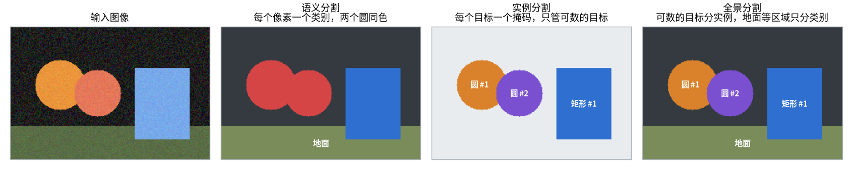
• 语义分割把两个相互接触的圆画成同一种颜色，只知道这些像素是圆，不知道有几个
• 实例分割可以看作检测的延伸：先找到每个目标，再在框内预测掩码。它只关心人、车这类可数的目标（things），天空、地面、道路这类不可数的区域（stuff）不输出
• 全景分割把两者合并：每个像素都有类别，属于可数目标的像素还有实例编号

本文以语义分割为主，它是另外两种任务的基础。实例分割在torchvision.models.detection中有maskrcnn_resnet50_fpn，输出格式与检测模型相同，只是每个目标多一个masks字段

标注与数据

示例数据集

下文用一个合成的数据集演示完整的流程：64x64 的噪声背景上随机画 1 到 3 个圆、矩形或三角形，颜色随机，模型只能从形状判断类别。数据集在内存中生成，不需要下载，保存为shapes.py供后面的代码导入

import cv2
import numpy as np
import torch
from torch.utils.data import Dataset

CLASSES = ['背景', '圆', '矩形', '三角形']


def make_sample(rng, size=64):
    """生成一张图像和它的掩码。image: (size, size, 3) uint8，mask: (size, size) uint8"""
    image = rng.integers(0, 80, (size, size, 3)).astype(np.uint8)  # 噪声背景
    mask = np.zeros((size, size), np.uint8)
    for _ in range(rng.integers(1, 4)):  # 1 到 3 个图形，后画的会遮挡先画的
        cls = int(rng.integers(1, 4))
        cx, cy = (int(v) for v in rng.integers(10, size - 10, 2))
        w, h = (int(v) for v in rng.integers(5, 10, 2))  # 半宽和半高
        shape = np.zeros((size, size), np.uint8)
        if cls == 1:
            cv2.circle(shape, (cx, cy), w, 1, -1)
        elif cls == 2:
            cv2.rectangle(shape, (cx - w, cy - h), (cx + w, cy + h), 1, -1)
        else:
            points = np.array([[cx, cy - h], [cx - w, cy + h], [cx + w, cy + h]])
            cv2.fillPoly(shape, [points], 1)
        # 颜色是随机的，类别只能从形状判断
        image[shape == 1] = rng.integers(120, 256, 3)
        mask[shape == 1] = cls
    noise = rng.normal(0, 12, image.shape)
    image = np.clip(image + noise, 0, 255).astype(np.uint8)
    return image, mask


class ShapesDataset(Dataset):
    def __init__(self, length, seed):
        rng = np.random.default_rng(seed)
        samples = [make_sample(rng) for _ in range(length)]
        self.images = np.stack([s[0] for s in samples])  # (length, 64, 64, 3) uint8
        self.masks = np.stack([s[1] for s in samples])   # (length, 64, 64) uint8

    def __len__(self):
        return len(self.images)

    def __getitem__(self, index):
        image = torch.from_numpy(self.images[index]).permute(2, 0, 1).float() / 255  # (3, 64, 64)，0 到 1
        mask = torch.from_numpy(self.masks[index]).long()                            # (64, 64)，int64
        return image, mask


if __name__ == '__main__':
    dataset = ShapesDataset(1600, seed=0)
    image, mask = dataset[0]
    print(image.shape, image.dtype)  # torch.Size([3, 64, 64]) torch.float32
    print(mask.shape, mask.dtype)    # torch.Size([64, 64]) torch.int64
    print(mask.unique())

    # 各个类别的像素所占的比例
    counts = np.bincount(dataset.masks.ravel(), minlength=len(CLASSES))
    for name, ratio in zip(CLASSES, counts / counts.sum()):
        print(f'{name} {ratio:.1%}')

torch.Size([3, 64, 64]) torch.float32
torch.Size([64, 64]) torch.int64
tensor([0, 1, 3])
背景 92.2%
圆 2.5%
矩形 3.4%
三角形 1.8%

背景占了 92% 的像素，这是分割数据的常态，后面的损失函数和评价指标都要考虑这一点

掩码的格式

格式	形状	数据类型	用途
类别索引图	(H, W)	整数，取值为类别编号	标注文件、cross_entropy的标签
one-hot	(C, H, W)	0 或 1	计算 Dice 损失、多标签分割
二值掩码	(H, W)	bool 或 0/1	单个类别或单个实例，实例分割的输出
调色板 PNG	(H, W)	uint8，带调色板	Pascal VOC 等数据集的标注文件

忽略标签通常取 255：图像边缘、目标之间难以判断的边界、旋转后填充的区域标为 255，计算损失和指标时跳过这些像素

import cv2
import numpy as np
import torch
import torch.nn.functional as F
from PIL import Image

from shapes import make_sample

image, mask = make_sample(np.random.default_rng(0))
print(image.shape, image.dtype)  # (64, 64, 3) uint8
print(mask.shape, mask.dtype)    # (64, 64) uint8
print(np.unique(mask))           # [0 1 3]，这张图像中有背景、圆和三角形

# 类别索引图 -> one-hot：(H, W) -> (H, W, C) -> (C, H, W)
index = torch.from_numpy(mask).long()
onehot = F.one_hot(index, num_classes=4).permute(2, 0, 1)
print(onehot.shape, onehot.dtype)             # torch.Size([4, 64, 64]) torch.int64
print(onehot.sum(dim=0).unique())             # tensor([1])，每个像素只属于一个类别
print(torch.equal(onehot.argmax(dim=0), index))  # True，argmax 可以还原

# 某一个类别的二值掩码
circle = index == 1
print(circle.shape, circle.dtype, circle.sum().item())

# 掩码必须用无损格式保存：JPEG 压缩会改变像素值，也就改变了类别编号
_, png = cv2.imencode('.png', mask)
_, jpg = cv2.imencode('.jpg', mask)
print(np.unique(cv2.imdecode(png, cv2.IMREAD_GRAYSCALE)))  # [0 1 3]
print(np.unique(cv2.imdecode(jpg, cv2.IMREAD_GRAYSCALE)))

# 调色板 PNG（Pascal VOC 的标注格式）：用 PIL 读到的是类别编号，用 OpenCV 读到的是颜色
palette = Image.fromarray(mask, mode='P')
palette.putpalette([0, 0, 0, 128, 0, 0, 0, 128, 0, 128, 128, 0])
palette.save('mask.png')
print(np.unique(np.array(Image.open('mask.png'))))                         # [0 1 3]
print(np.unique(cv2.imread('mask.png').reshape(-1, 3), axis=0).tolist())  # BGR 颜色

(64, 64, 3) uint8
(64, 64) uint8
[0 1 3]
torch.Size([4, 64, 64]) torch.int64
tensor([1])
True
torch.Size([64, 64]) torch.bool 219
[0 1 3]
[0 1 2 3 4]
[0 1 3]
[[0, 0, 0], [0, 0, 128], [0, 128, 128]]

• 用 JPEG 保存的掩码读回来多出了 2 和 4 两个类别：有损压缩会在边界附近产生新的像素值，掩码必须保存为 PNG
• 调色板 PNG 中存的是类别编号，显示出来是彩色的。用PIL读取得到编号；用cv2.imread读取会按调色板转换成 BGR 颜色，得到的不是类别编号

插值方式

缩放图像时常用双线性插值，它在相邻像素之间取加权平均。对掩码这样做，两个类别的交界处会出现介于两者之间的数值，取整后就是其他类别的编号

import torch
import torch.nn.functional as F
from torchvision import tv_tensors
from torchvision.transforms import v2

# 只有背景（0）和三角形（3）两个类别的掩码
mask = torch.zeros(64, 64, dtype=torch.uint8)
mask[16:48, 16:48] = 3

# 错误：按图像的方式用双线性插值放大
x = mask[None, None].float()  # interpolate 要求 (N, C, H, W) 的浮点张量
bilinear = F.interpolate(x, size=(100, 100), mode='bilinear', align_corners=False).round().long()
print(bilinear.unique().tolist(), torch.bincount(bilinear.flatten()).tolist())

# 正确：最近邻插值
nearest = F.interpolate(x, size=(100, 100), mode='nearest').long()
print(nearest.unique().tolist(), torch.bincount(nearest.flatten()).tolist())

# torchvision 的变换把普通张量当作图像处理，同样是双线性插值
print(v2.functional.resize(mask[None], [100, 100]).unique().tolist())
# 包装成 tv_tensors.Mask 之后自动使用最近邻插值
print(v2.functional.resize(tv_tensors.Mask(mask), [100, 100]).unique().tolist())

[0, 1, 2, 3] [7308, 192, 196, 2304]
[0, 3] [7500, 0, 0, 2500]
[0, 1, 2, 3]
[0, 3]

原本只有背景（0）和三角形（3）的掩码，用双线性插值放大后，在两者的交界处多出了 192 个标为 1（圆）和 196 个标为 2（矩形）的像素，模型会被要求在三角形的边上预测出圆和矩形。最近邻插值只会复制已有的值，不会产生新的类别

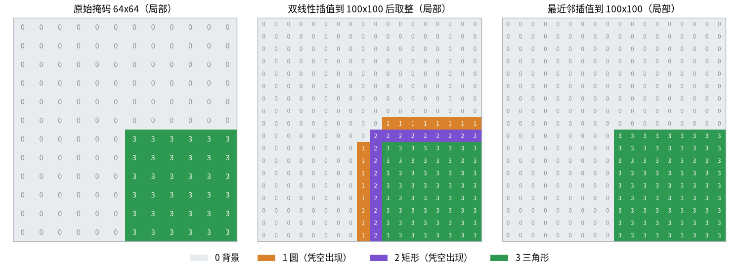
torchvision.transforms.v2根据输入的类型决定插值方式：普通张量和tv_tensors.Image当作图像，用双线性插值；tv_tensors.Mask当作掩码，自动改用最近邻插值

同步的几何变换

数据增强中的几何变换（裁剪、翻转、旋转、缩放）必须对图像和掩码使用同一组随机参数，颜色变换（亮度、对比度、模糊）只作用于图像。transforms.v2的做法是把图像和掩码在同一次调用中传入，各自包装成对应的tv_tensors类型

import numpy as np
import torch
from torchvision import tv_tensors
from torchvision.transforms import v2

from shapes import make_sample

image, mask = make_sample(np.random.default_rng(0))
image = tv_tensors.Image(torch.from_numpy(image).permute(2, 0, 1))  # (3, 64, 64) uint8
mask = tv_tensors.Mask(torch.from_numpy(mask))                      # (64, 64) uint8

transform = v2.Compose([
    v2.RandomResizedCrop(64, scale=(0.5, 1.0)),  # 几何变换：图像和掩码使用同一组随机参数
    v2.RandomHorizontalFlip(),
    v2.RandomRotation(15, fill={ tv_tensors.Image: 0, tv_tensors.Mask: 255 }),  # 旋转后露出的区域在掩码中填 255
    v2.ColorJitter(brightness=0.3, contrast=0.3),  # 颜色变换：只作用于图像
    v2.ToDtype({ tv_tensors.Image: torch.float32, tv_tensors.Mask: torch.int64 }, scale=True),
])

torch.manual_seed(0)
out_image, out_mask = transform(image, mask)
print(type(out_image).__name__, out_image.shape, out_image.dtype)
print(type(out_mask).__name__, out_mask.shape, out_mask.dtype)
print(mask.unique().tolist(), '->', out_mask.unique().tolist())



def agreement(image, mask):
    """图形比背景亮：统计“像素是否明亮”与“掩码是否为前景”一致的比例，用来检查图像和掩码是否对齐"""
    bright = image.max(dim=0).values > 115
    return ((mask > 0) == bright).float().mean().item()


print(f'{agreement(image, mask):.4f}')

# 正确：图像和掩码一起传入，使用同一组随机参数
crop = v2.RandomCrop(32)
torch.manual_seed(0)
crop_image, crop_mask = crop(image, mask)
print(f'{agreement(crop_image, crop_mask):.4f}')

# 错误 1：对图像和掩码分别调用，两次调用的随机参数不同
torch.manual_seed(0)
crop_image, crop_mask = crop(image), crop(mask)
print(f'{agreement(crop_image, crop_mask):.4f}')

# 错误 2：掩码是普通张量。有 tv_tensors.Image 在场时，其余的普通张量被原样返回，不做任何变换
flip = v2.RandomHorizontalFlip(p=1.0)
plain_mask = mask.as_subclass(torch.Tensor)
flip_image, flip_mask = flip(image, plain_mask)
print(torch.equal(flip_mask, plain_mask), f'{agreement(flip_image, flip_mask):.4f}')

Image torch.Size([3, 64, 64]) torch.float32
Mask torch.Size([64, 64]) torch.int64
[0, 1, 3] -> [0, 1, 3, 255]
1.0000
1.0000
0.8428
True 0.7627

• ToDtype对图像缩放到 0 到 1 的浮点数，对掩码只转换类型（int64是cross_entropy要求的标签类型），scale=True不会作用于掩码
• 旋转后露出的角落在图像中填 0，在掩码中填 255。如果掩码也填 0，这些黑色区域会被当作背景参与训练
• agreement检查的是图形区域与掩码前景是否重合，原图上为 1。一起传入时裁剪后仍然是 1；分别调用时两次裁剪的位置不同，降到 0.8428
• 普通张量和tv_tensors.Image一起传入时，transforms.v2把普通张量当作不需要变换的附加数据原样返回。图像翻转了，掩码没有，也不会有任何警告

这类错误不会报错，训练也能进行，只是指标始终上不去。 写好数据管道后，把增强后的图像和掩码叠加画出来检查一遍，比任何单元测试都直接

模型结构

编码器与解码器

分类网络通过不断下采样得到一个全局的特征向量，分割需要的是与输入同样大小的输出。分割网络通常分为两部分：

部分	作用	分辨率的变化
编码器	提取特征，通常就是去掉分类头的分类网络	逐步缩小
解码器	把特征放大回输入的分辨率，对每个像素做分类	逐步放大

深层特征语义强但分辨率低，直接放大 8 倍或 32 倍得到的边界很粗糙。U-Net 在每一次上采样之后，把编码器中同分辨率的浅层特征拼接进来，用来恢复细节。上采样与拼接的形状计算见PyTorch CNN中的上采样拼接一节

一个小型 U-Net

下面的 U-Net 有 3 次下采样，基础通道数为 16。最后的 1x1 卷积把通道数变为类别数，输出形状为 (N, C, H, W)，即每个像素一组未归一化的分数（logits）

import torch
import torch.nn as nn


class DoubleConv(nn.Sequential):
    """两个 3x3 卷积，不改变高度和宽度"""

    def __init__(self, in_channels, out_channels):
        super().__init__(
            nn.Conv2d(in_channels, out_channels, 3, padding=1, bias=False),
            nn.BatchNorm2d(out_channels),
            nn.ReLU(inplace=True),
            nn.Conv2d(out_channels, out_channels, 3, padding=1, bias=False),
            nn.BatchNorm2d(out_channels),
            nn.ReLU(inplace=True),
        )


class UpBlock(nn.Module):
    def __init__(self, in_channels, skip_channels, out_channels):
        super().__init__()
        self.up = nn.ConvTranspose2d(in_channels, in_channels // 2, kernel_size=2, stride=2)
        self.conv = DoubleConv(in_channels // 2 + skip_channels, out_channels)

    def forward(self, x, skip):
        x = self.up(x)                   # 高度和宽度放大 2 倍
        x = torch.cat([x, skip], dim=1)  # 与编码器中同分辨率的特征拼接
        return self.conv(x)


class UNet(nn.Module):
    def __init__(self, in_channels=3, num_classes=4, base=16):
        super().__init__()
        # 编码器：每下采样一次，通道数翻倍
        self.enc1 = DoubleConv(in_channels, base)
        self.enc2 = DoubleConv(base, base * 2)
        self.enc3 = DoubleConv(base * 2, base * 4)
        self.bottleneck = DoubleConv(base * 4, base * 8)
        self.pool = nn.MaxPool2d(2)
        # 解码器：每上采样一次，通道数减半
        self.dec3 = UpBlock(base * 8, base * 4, base * 4)
        self.dec2 = UpBlock(base * 4, base * 2, base * 2)
        self.dec1 = UpBlock(base * 2, base, base)
        # 1x1 卷积把通道数变为类别数，每个像素得到一组分类的 logits
        self.head = nn.Conv2d(base, num_classes, kernel_size=1)

    def forward(self, x):
        e1 = self.enc1(x)                     # (N, 16, H, W)
        e2 = self.enc2(self.pool(e1))         # (N, 32, H/2, W/2)
        e3 = self.enc3(self.pool(e2))         # (N, 64, H/4, W/4)
        b = self.bottleneck(self.pool(e3))    # (N, 128, H/8, W/8)
        d3 = self.dec3(b, e3)                 # (N, 64, H/4, W/4)
        d2 = self.dec2(d3, e2)                # (N, 32, H/2, W/2)
        d1 = self.dec1(d2, e1)                # (N, 16, H, W)
        return self.head(d1)                  # (N, num_classes, H, W)


if __name__ == '__main__':
    model = UNet()
    x = torch.randn(2, 3, 64, 64)
    print(model(x).shape)  # torch.Size([2, 4, 64, 64])
    print(sum(p.numel() for p in model.parameters()))

    # 高度和宽度必须能被 8 整除（3 次下采样），否则拼接时尺寸对不上
    try:
        model(torch.randn(2, 3, 100, 100))
    except RuntimeError as e:
        print(e)

torch.Size([2, 4, 64, 64])
482788
Sizes of tensors must match except in dimension 1. Expected size 24 but got size 25 for tensor number 1 in the list.

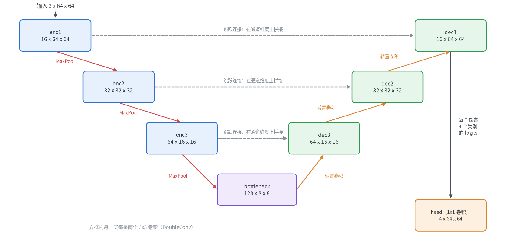
100x100 的输入在第 3 次池化后变成 12x12，放大回来是 24x24，与编码器中 25x25 的特征无法拼接。常见的处理方式是把输入填充到 8 的倍数，推理后再裁掉；或者在拼接前用F.interpolate把上采样的结果缩放到与跳跃连接相同的尺寸

其他结构与 torchvision 中的模型

结构	思路
FCN	把分类网络的全连接层换成卷积，直接把最后的特征图放大到原图
U-Net	对称的编码器和解码器，每一级都有跳跃连接，适合小数据集
DeepLab	用空洞卷积代替部分下采样，ASPP 模块用不同膨胀率的卷积并行提取多尺度特征
LR-ASPP	为 MobileNetV3 设计的轻量分割头，适合移动端

torchvision.models.segmentation中提供的预训练模型：

函数	骨干网络	输出字典中的键
fcn_resnet50、fcn_resnet101	ResNet	out、aux
deeplabv3_resnet50、deeplabv3_resnet101	ResNet	out、aux
deeplabv3_mobilenet_v3_large	MobileNetV3-Large	out、aux
lraspp_mobilenet_v3_large	MobileNetV3-Large	out

它们的预训练权重都是在 COCO 的子集上按 Pascal VOC 的 20 个类别训练的，用法见最后一节

损失函数

像素级交叉熵

分割的交叉熵就是对每个像素分别计算分类的交叉熵，再取平均。F.cross_entropy直接支持多维输入，对形状的要求如下

参数	形状	数据类型	说明
input	(N, C, H, W)	浮点	网络输出的 logits，不做 softmax
target	(N, H, W)	int64	类别编号，没有通道维度
weight	(C,)	浮点	每个类别的权重，可选

import torch
import torch.nn.functional as F

torch.manual_seed(0)
logits = torch.randn(2, 4, 64, 64)         # 网络输出 (N, C, H, W)，不要先做 softmax
target = torch.randint(0, 4, (2, 64, 64))  # 标签 (N, H, W)，int64，取值为类别编号

print(F.cross_entropy(logits, target))

# 常见的形状和类型错误
for name, wrong in [('多了通道维度', target[:, None]), ('uint8', target.to(torch.uint8)), ('float32', target.float())]:
    try:
        F.cross_entropy(logits, wrong)
    except Exception as e:
        print(f'{name}: {type(e).__name__}: {str(e).splitlines()[0]}')

# 忽略标签：把一部分像素标为 255
ignored = target.clone()
ignored[:, :16] = 255
try:
    F.cross_entropy(logits, ignored)
except Exception as e:
    print(f'{type(e).__name__}: {e}')
loss = F.cross_entropy(logits, ignored, ignore_index=255)
print(loss)
# 等价于只在没有被忽略的像素上取平均
per_pixel = F.cross_entropy(logits, ignored, ignore_index=255, reduction='none')  # (N, H, W)，被忽略的位置为 0
print(per_pixel.shape, per_pixel[ignored != 255].mean())

# 类别权重：取平均时除以的是权重之和，不是像素数
weight = torch.tensor([0.2, 1.0, 1.0, 1.0])
weighted = F.cross_entropy(logits, target, weight=weight)
per_pixel = F.cross_entropy(logits, target, weight=weight, reduction='none')
print(weighted, per_pixel.sum() / weight[target].sum())

tensor(1.7180)
多了通道维度: RuntimeError: only batches of spatial targets supported (3D tensors) but got targets of dimension: 4
uint8: RuntimeError: expected scalar type Long but found Byte
float32: RuntimeError: expected target dtype to be Long or Byte, but got Float
IndexError: Target 255 is out of bounds.
tensor(1.7132)
torch.Size([2, 64, 64]) tensor(1.7132)
tensor(1.7150) tensor(1.7150)

• 从数据集中读出的掩码常常是 (N, 1, H, W) 或uint8，要先squeeze(1)并转成long()
• 标签中有 255 而没有设置ignore_index时会直接报错；ignore_index的默认值是 -100，不是 255，需要显式传入
• 设置了weight之后，reduction='mean'除以的是这些像素的权重之和，不是像素数

前景很小时

前景只占很小比例时，交叉熵的大部分可以靠把背景预测对来降低。下面构造一个前景只占 0.88% 的二分类例子，比较几种预测下的交叉熵和 Dice 损失。Dice 损失是 1 减去 Dice 系数，对每个类别分别计算再取平均，用概率代替 0/1 的预测使它可导，保存为losses.py

import torch
import torch.nn.functional as F


def dice_loss(logits, target, ignore_index=255, eps=1.0):
    """logits: (N, C, H, W)，target: (N, H, W)。对每个类别计算 Dice，再对类别取平均"""
    num_classes = logits.shape[1]
    valid = target != ignore_index                                # (N, H, W)
    prob = logits.softmax(dim=1) * valid[:, None]                 # 被忽略的像素不参与计算
    onehot = F.one_hot(target * valid, num_classes).permute(0, 3, 1, 2) * valid[:, None]
    inter = (prob * onehot).sum(dim=(0, 2, 3))                    # (C,)，在整个批次上求和
    total = prob.sum(dim=(0, 2, 3)) + onehot.sum(dim=(0, 2, 3))
    dice = (2 * inter + eps) / (total + eps)                      # eps 避免某个类别不存在时出现 0/0
    return 1 - dice.mean()

import torch
import torch.nn.functional as F

from losses import dice_loss


def report(name, logits, target):
    ce = F.cross_entropy(logits, target, reduction='none')
    accuracy = (logits.argmax(dim=1) == target).float().mean()
    foreground_share = ce[target == 1].sum() / ce.sum()
    print(f'{name}  准确率 {accuracy:.4f}  交叉熵 {ce.mean():.4f}（前景像素贡献 {foreground_share:.1%}）  Dice 损失 {dice_loss(logits, target):.4f}')


# 二分类，64x64 的图像中前景只有一个 6x6 的方块，占 0.88%
target = torch.zeros(1, 64, 64, dtype=torch.long)
target[:, 20:26, 20:26] = 1
print(f'{target.float().mean():.4f}')


def make_logits(foreground_mask, margin=8.0):
    """在 foreground_mask 为 True 的位置预测前景，其余位置预测背景，两个类别的 logit 相差 margin"""
    logits = torch.zeros(1, 2, 64, 64)
    logits[:, 0] = torch.where(foreground_mask, -margin / 2, margin / 2)
    logits[:, 1] = -logits[:, 0]
    return logits


half = torch.zeros_like(target, dtype=torch.bool)
half[:, 20:26, 20:23] = True

report('输出均匀  ', torch.zeros(1, 2, 64, 64), target)
report('全预测背景', make_logits(torch.zeros_like(half)), target)
report('找到一半  ', make_logits(half), target)
report('完全正确  ', make_logits(target == 1), target)

0.0088
输出均匀    准确率 0.9912  交叉熵 0.6931（前景像素贡献 0.9%）  Dice 损失 0.6587
全预测背景  准确率 0.9912  交叉熵 0.0706（前景像素贡献 99.5%）  Dice 损失 0.4889
找到一半    准确率 0.9956  交叉熵 0.0355（前景像素贡献 99.1%）  Dice 损失 0.1730
完全正确    准确率 1.0000  交叉熵 0.0003（前景像素贡献 0.9%）  Dice 损失 0.0093

• 从均匀的输出到全部预测为背景，交叉熵从 0.6931 降到 0.0706，已经走完了 90% 的路，而一个前景像素都没有找到。准确率也已经是 0.9912
• Dice 损失对类别取平均，前景这个类别和背景的权重相同。全预测背景时前景的 Dice 是 0，损失仍有 0.4889

下面在真实的训练中验证这一点：每张 64x64 的图像中只有一个半径为 2 的圆点，前景占 0.32%，分别只用交叉熵和用交叉熵加 Dice 损失训练同一个 U-Net

import cv2
import numpy as np
import torch
import torch.nn.functional as F

from losses import dice_loss
from unet import UNet


def make_data(length, seed):
    """单通道的噪声图像，每张图像中有一个半径为 2 的圆点，只比背景略亮"""
    rng = np.random.default_rng(seed)
    images = rng.normal(0.3, 0.1, (length, 1, 64, 64)).astype(np.float32)
    masks = np.zeros((length, 64, 64), np.int64)
    for i in range(length):
        cx, cy = (int(v) for v in rng.integers(5, 59, 2))
        dot = cv2.circle(np.zeros((64, 64), np.uint8), (cx, cy), 2, 1, -1)
        images[i, 0][dot == 1] += 0.15
        masks[i] = dot
    return torch.from_numpy(images), torch.from_numpy(masks)


train_images, train_masks = make_data(1024, seed=0)
val_images, val_masks = make_data(256, seed=1)
print(f'前景像素占比 {train_masks.float().mean():.2%}')

for use_dice in [False, True]:
    torch.manual_seed(0)
    model = UNet(in_channels=1, num_classes=2, base=8)
    optimizer = torch.optim.AdamW(model.parameters(), lr=1e-3)
    for step in range(1, 641):
        index = torch.randint(0, len(train_images), (32,))
        model.train()
        logits = model(train_images[index])
        loss = F.cross_entropy(logits, train_masks[index])
        if use_dice:
            loss = loss + dice_loss(logits, train_masks[index])
        optimizer.zero_grad()
        loss.backward()
        optimizer.step()

        if step % 160 == 0:
            model.eval()
            with torch.no_grad():
                pred = model(val_images).argmax(dim=1)
            accuracy = (pred == val_masks).float().mean()
            inter = ((pred == 1) & (val_masks == 1)).sum()
            union = ((pred == 1) | (val_masks == 1)).sum()
            print(f'{"交叉熵 + Dice" if use_dice else "交叉熵       "}  step {step:3d}  '
                  f'像素准确率 {accuracy:.4f}  前景 IoU {inter / union:.4f}  预测为前景的像素 {(pred == 1).sum().item()}')

前景像素占比 0.32%
交叉熵         step 160  像素准确率 0.9968  前景 IoU 0.0056  预测为前景的像素 58
交叉熵         step 320  像素准确率 0.9968  前景 IoU 0.0000  预测为前景的像素 0
交叉熵         step 480  像素准确率 0.9968  前景 IoU 0.0000  预测为前景的像素 0
交叉熵         step 640  像素准确率 0.9968  前景 IoU 0.0000  预测为前景的像素 0
交叉熵 + Dice  step 160  像素准确率 0.9968  前景 IoU 0.0565  预测为前景的像素 377
交叉熵 + Dice  step 320  像素准确率 0.9969  前景 IoU 0.4753  预测为前景的像素 5791
交叉熵 + Dice  step 480  像素准确率 0.9984  前景 IoU 0.6205  预测为前景的像素 3627
交叉熵 + Dice  step 640  像素准确率 0.9992  前景 IoU 0.7859  预测为前景的像素 3412

只用交叉熵时，模型很快退化成把所有像素都预测为背景，像素准确率停在 0.9968，正好等于背景所占的比例。加上 Dice 损失后，前景 IoU 达到 0.7859。把随机种子换成 1 和 2 再各跑一次，只用交叉熵时 3 次中有 1 次在 640 步时学到了前景（IoU 0.5672），另外 2 次都是全预测背景；加上 Dice 损失的 3 次分别为 0.7859、0.7426、0.7440

处理前景过少的常用方法：

方法	做法
交叉熵 + Dice	两者直接相加，交叉熵提供稳定的逐像素梯度，Dice 照顾小类别
类别权重	cross_entropy的weight，常取类别频率的倒数或其平方根
Focal Loss	降低已经分对的像素的权重，见Object Detection
采样	裁剪训练图像时优先选择包含前景的区域

Dice 损失单独使用时训练初期不稳定，实践中最常见的组合是交叉熵加 Dice。上一节形状数据集的前景约占 8%，并不算极端，在同样的设置下只用交叉熵训练 8 个 epoch 的 mIoU 为 0.9727，只用 Dice 为 0.9713，两者相加为 0.9742，差别不大

训练

训练循环与分类任务相同（DataLoader 的写法见PyTorch Data Loading，优化器、学习率调度的写法见PyTorch Training），区别只在于输出和标签都是逐像素的。在形状数据集上用交叉熵加 Dice 损失训练 8 个 epoch，每个 epoch 结束后在验证集上累积混淆矩阵，计算像素准确率和 mIoU

import json

import torch
import torch.nn.functional as F
from torch.utils.data import DataLoader

from losses import dice_loss
from shapes import CLASSES, ShapesDataset
from unet import UNet


@torch.no_grad()
def evaluate(model, loader, num_classes):
    """累积整个验证集的混淆矩阵，返回像素准确率和各类别的 IoU"""
    model.eval()
    matrix = torch.zeros(num_classes, num_classes, dtype=torch.long)  # 行是真实类别，列是预测类别
    for images, masks in loader:
        preds = model(images).argmax(dim=1)
        matrix += torch.bincount(masks.flatten() * num_classes + preds.flatten(),
                                 minlength=num_classes ** 2).view(num_classes, num_classes)
    tp = matrix.diag()
    accuracy = tp.sum() / matrix.sum()
    iou = tp / (matrix.sum(0) + matrix.sum(1) - tp)
    return accuracy.item(), iou


if __name__ == '__main__':
    torch.manual_seed(0)
    train_loader = DataLoader(ShapesDataset(1600, seed=0), batch_size=32, shuffle=True)
    val_loader = DataLoader(ShapesDataset(400, seed=1), batch_size=100)

    epochs = 8
    model = UNet(num_classes=len(CLASSES))
    optimizer = torch.optim.AdamW(model.parameters(), lr=3e-3, weight_decay=1e-4)
    scheduler = torch.optim.lr_scheduler.OneCycleLR(optimizer, max_lr=3e-3, total_steps=epochs * len(train_loader))

    history = { 'loss': [], 'accuracy': [], 'miou': [], 'iou': [] }
    for epoch in range(epochs):
        model.train()
        for images, masks in train_loader:
            logits = model(images)  # (N, 4, 64, 64)
            loss = F.cross_entropy(logits, masks) + dice_loss(logits, masks)
            optimizer.zero_grad()
            loss.backward()
            optimizer.step()
            scheduler.step()
            history['loss'].append(loss.item())

        accuracy, iou = evaluate(model, val_loader, len(CLASSES))
        history['accuracy'].append(accuracy)
        history['miou'].append(iou.mean().item())
        history['iou'].append(iou.tolist())
        print(f'epoch {epoch + 1:2d}  loss {loss.item():.4f}  像素准确率 {accuracy:.4f}  mIoU {iou.mean():.4f}')

    torch.save(model.state_dict(), 'unet.pt')
    json.dump(history, open('history.json', 'w'))

epoch  1  loss 2.0852  像素准确率 0.2488  mIoU 0.0705
epoch  2  loss 1.2556  像素准确率 0.9706  mIoU 0.7449
epoch  3  loss 0.1984  像素准确率 0.9911  mIoU 0.8255
epoch  4  loss 0.0903  像素准确率 0.9983  mIoU 0.9691
epoch  5  loss 0.0497  像素准确率 0.9981  mIoU 0.9649
epoch  6  loss 0.0401  像素准确率 0.9986  mIoU 0.9731
epoch  7  loss 0.0370  像素准确率 0.9986  mIoU 0.9741
epoch  8  loss 0.0404  像素准确率 0.9986  mIoU 0.9742

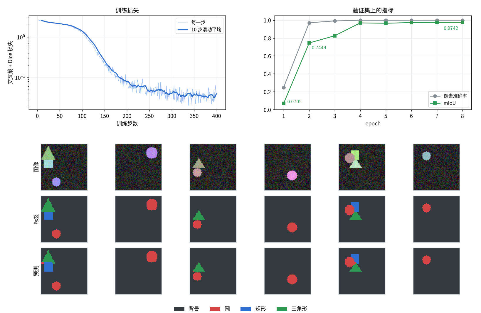
第 2 个 epoch 结束时像素准确率已经是 0.9706，mIoU 只有 0.7449；第 3 个 epoch 像素准确率 0.9911，看起来几乎完美，mIoU 仍只有 0.8255。预测结果中的错误主要在图形的边缘和两个图形相互遮挡的地方

评价指标

IoU、Dice 和 mIoU 的定义、由混淆矩阵计算 mIoU 的方法见Evaluation Metrics。这里用训练好的模型比较三个指标，并加上一个把所有像素都预测为背景的基线

import torch
from torch.utils.data import DataLoader

from shapes import CLASSES, ShapesDataset
from unet import UNet

num_classes = len(CLASSES)
model = UNet(num_classes=num_classes)
model.load_state_dict(torch.load('unet.pt'))
model.eval()

loader = DataLoader(ShapesDataset(400, seed=1), batch_size=100)


def metrics(matrix):
    tp = matrix.diag().float()
    accuracy = tp.sum() / matrix.sum()
    iou = tp / (matrix.sum(0) + matrix.sum(1) - tp)
    dice = 2 * tp / (matrix.sum(0) + matrix.sum(1))
    return accuracy, iou, dice


# 在整个验证集上累积两个混淆矩阵：一个是模型的预测，一个是把所有像素都预测为背景
matrix = torch.zeros(num_classes, num_classes, dtype=torch.long)
baseline = torch.zeros(num_classes, num_classes, dtype=torch.long)
with torch.no_grad():
    for images, masks in loader:
        preds = model(images).argmax(dim=1)
        matrix += torch.bincount(masks.flatten() * num_classes + preds.flatten(),
                                 minlength=num_classes ** 2).view(num_classes, num_classes)
        baseline[:, 0] += torch.bincount(masks.flatten(), minlength=num_classes)

print(matrix)
for name, m in [('全预测背景', baseline), ('U-Net', matrix)]:
    accuracy, iou, dice = metrics(m)
    print(f'{name}  像素准确率 {accuracy:.4f}  mIoU {iou.mean():.4f}  平均 Dice {dice.mean():.4f}')
    print('  IoU  ', '  '.join(f'{c} {v:.4f}' for c, v in zip(CLASSES, iou.tolist())))
    print('  Dice ', '  '.join(f'{c} {v:.4f}' for c, v in zip(CLASSES, dice.tolist())))

tensor([[1506581,       2,       0,       0],
        [     14,   42629,     412,     136],
        [     27,     597,   58550,     303],
        [     13,     287,     461,   28388]])
全预测背景  像素准确率 0.9195  mIoU 0.2299  平均 Dice 0.2395
  IoU   背景 0.9195  圆 0.0000  矩形 0.0000  三角形 0.0000
  Dice  背景 0.9581  圆 0.0000  矩形 0.0000  三角形 0.0000
U-Net  像素准确率 0.9986  mIoU 0.9742  平均 Dice 0.9869
  IoU   背景 1.0000  圆 0.9671  矩形 0.9702  三角形 0.9594
  Dice  背景 1.0000  圆 0.9833  矩形 0.9849  三角形 0.9793

指标	全预测背景	U-Net	说明
像素准确率	0.9195	0.9986	被背景主导，什么都不做也有 0.92
mIoU	0.2299	0.9742	每个类别权重相同，能反映前景的好坏
平均 Dice	0.2395	0.9869	与 mIoU 单调对应，数值总是更高

• 混淆矩阵中前景之间的混淆（圆被预测为矩形 412 个像素，矩形被预测为圆 597 个像素）远多于前景与背景之间的混淆，说明模型找到了图形的位置，错误主要在相互遮挡处的类别判断
• 报告结果时 mIoU 和平均 Dice 要写明是哪一个，是否包含背景类。去掉背景类后，U-Net 的 mIoU 为三个前景类别的平均值 0.9656
• 指标要在整个验证集上累积混淆矩阵之后再计算，不能对每个批次或每张图像的 mIoU 取平均

推理与后处理

从 logits 到类别图

推理时对类别维度取argmax得到类别图。输入图像常常需要缩放后才能送入网络，结果需要还原到原图尺寸，这时应当先用双线性插值放大 logits，再取argmax；先取argmax再用最近邻插值放大类别图，边界会呈锯齿状

下面用一张 256x256 的图像，把它缩小到训练时的 64x64 再预测，然后还原到原图尺寸，并把结果拆成单个的目标

import cv2
import numpy as np
import torch
import torch.nn.functional as F

from shapes import CLASSES
from unet import UNet

# 一张 256x256 的图像：两个圆、两个相邻的矩形、一个三角形
rng = np.random.default_rng(0)
image = rng.integers(0, 80, (256, 256, 3)).astype(np.uint8)
truth = np.zeros((256, 256), np.uint8)
for cls, color, draw in [
    (1, (235, 150, 60), lambda m: cv2.circle(m, (56, 56), 28, 1, -1)),
    (1, (120, 200, 230), lambda m: cv2.circle(m, (200, 60), 24, 1, -1)),
    (2, (200, 130, 220), lambda m: cv2.rectangle(m, (24, 150), (88, 214), 1, -1)),
    (2, (230, 220, 120), lambda m: cv2.rectangle(m, (89, 170), (136, 230), 1, -1)),
    (3, (140, 230, 150), lambda m: cv2.fillPoly(m, [np.array([[196, 130], [150, 222], [242, 222]])], 1)),
]:
    shape = draw(np.zeros((256, 256), np.uint8))
    image[shape == 1] = color
    truth[shape == 1] = cls
image = np.clip(image + rng.normal(0, 12, image.shape), 0, 255).astype(np.uint8)

model = UNet(num_classes=len(CLASSES))
model.load_state_dict(torch.load('unet.pt'))
model.eval()

# 模型在 64x64 的图像上训练，先把图像缩小再送入网络
small = cv2.resize(image, (64, 64), interpolation=cv2.INTER_AREA)
x = torch.from_numpy(small).permute(2, 0, 1).float()[None] / 255
with torch.no_grad():
    logits = model(x)  # (1, 4, 64, 64)


def mean_iou(pred, truth, num_classes=4):
    ious = [((pred == c) & (truth == c)).sum() / ((pred == c) | (truth == c)).sum() for c in range(num_classes)]
    return float(np.mean(ious))


# 做法 1：先把 logits 用双线性插值放大到原图尺寸，再取 argmax
upsampled = F.interpolate(logits, size=(256, 256), mode='bilinear', align_corners=False)
pred = upsampled.argmax(dim=1)[0].numpy().astype(np.uint8)  # (256, 256)
# 做法 2：先取 argmax，再把类别图用最近邻插值放大
coarse = logits.argmax(dim=1)[0].numpy().astype(np.uint8)   # (64, 64)
pred_nearest = cv2.resize(coarse, (256, 256), interpolation=cv2.INTER_NEAREST)
print(f'放大 logits   mIoU {mean_iou(pred, truth):.4f}')
print(f'放大类别图    mIoU {mean_iou(pred_nearest, truth):.4f}')


# 连通域：把每个类别的二值掩码拆成互不相连的区域
instances = []
for cls in range(1, len(CLASSES)):
    binary = (pred == cls).astype(np.uint8)
    count, labels, stats, centroids = cv2.connectedComponentsWithStats(binary, connectivity=8)
    for i in range(1, count):  # 编号 0 是这张二值图的背景
        x0, y0, w, h, area = stats[i].tolist()
        if area < 50:          # 丢弃零碎的小区域
            continue
        # 轮廓：区域边界上的点，形状为 (点数, 1, 2)，坐标顺序为 (x, y)
        contours, _ = cv2.findContours((labels == i).astype(np.uint8), cv2.RETR_EXTERNAL, cv2.CHAIN_APPROX_SIMPLE)
        instances.append((cls, (x0, y0, w, h), area, contours[0]))
        print(f'{CLASSES[cls]}  框 (x, y, w, h) = {(x0, y0, w, h)}  面积 {area}  轮廓点数 {len(contours[0])}')

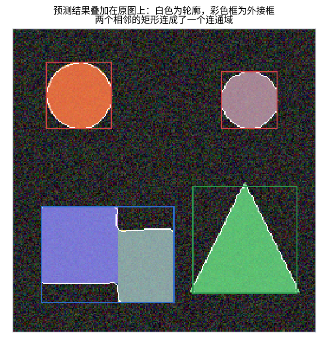
# 叠加显示：前景像素与类别颜色各占一半，再画出轮廓和外接框
palette = np.array([[0, 0, 0], [214, 69, 69], [47, 111, 208], [46, 153, 80]], np.uint8)  # 每个类别的 RGB 颜色
overlay = image.copy()
foreground = pred > 0
overlay[foreground] = (0.5 * image[foreground] + 0.5 * palette[pred][foreground]).astype(np.uint8)
for cls, (x0, y0, w, h), area, contour in instances:
    cv2.drawContours(overlay, [contour], -1, (255, 255, 255), 1)
    cv2.rectangle(overlay, (x0, y0), (x0 + w - 1, y0 + h - 1), palette[cls].tolist(), 1)
cv2.imwrite('overlay.png', cv2.cvtColor(overlay, cv2.COLOR_RGB2BGR))  # OpenCV 按 BGR 顺序保存

放大 logits   mIoU 0.9758
放大类别图    mIoU 0.9479
圆  框 (x, y, w, h) = (28, 28, 56, 57)  面积 2440  轮廓点数 84
圆  框 (x, y, w, h) = (176, 36, 48, 49)  面积 1859  轮廓点数 53
矩形  框 (x, y, w, h) = (24, 150, 113, 82)  面积 7261  轮廓点数 35
三角形  框 (x, y, w, h) = (152, 133, 89, 91)  面积 4444  轮廓点数 116

• 放大 logits 的 mIoU 为 0.9758，放大类别图为 0.9479。logits 是连续的，插值后再比较大小，相当于在像素之间估计边界的位置
• 每个类别的二值掩码用cv2.connectedComponentsWithStats拆成连通域，stats的每一行是[x, y, w, h, 面积]，可以直接作为检测框使用。面积过小的连通域通常是噪声，按阈值丢弃
• cv2.findContours返回每个区域的边界点，用于绘制、计算周长或转换成多边形格式的标注
• 两个相邻的矩形被合并成了一个连通域（框的宽度为 113）。语义分割本身不区分同类的不同个体，相互接触的同类目标无法靠连通域拆开，需要实例分割

常用的后处理

操作	做法	用途
去除小区域	连通域面积小于阈值的改为背景	去掉零散的误检
填充孔洞	形态学闭运算（cv2.morphologyEx）	让掩码内部连续
置信度阈值	softmax 的最大值低于阈值的像素标为不确定	只保留有把握的结果
掩码转多边形	cv2.findContours后用cv2.approxPolyDP简化	导出标注、矢量化

使用预训练模型

torchvision.models.segmentation中的模型返回一个字典，out是主输出，aux是训练时用于辅助损失的分支，推理时只用out。权重对象中带有类别列表和预处理方式。下面用 scikit-learn 自带的两张示例图像测试fcn_resnet50

import torch
import torch.nn.functional as F
from sklearn.datasets import load_sample_image
from torchvision.models.segmentation import FCN_ResNet50_Weights, fcn_resnet50

weights = FCN_ResNet50_Weights.DEFAULT
model = fcn_resnet50(weights=weights)
model.eval()

categories = weights.meta['categories']
print(len(categories), categories)
preprocess = weights.transforms()  # 缩放到短边 520，除以 255，按 ImageNet 的均值和标准差归一化
print(preprocess)

for name in ['china.jpg', 'flower.jpg']:
    image = torch.from_numpy(load_sample_image(name).copy()).permute(2, 0, 1)  # (3, 427, 640) uint8
    batch = preprocess(image).unsqueeze(0)
    with torch.no_grad():
        output = model(batch)  # 一个字典
    print(name, tuple(image.shape), '->', tuple(batch.shape), { k: tuple(v.shape) for k, v in output.items() })

    # 把 logits 缩放回原图尺寸，再取类别和置信度
    logits = F.interpolate(output['out'], size=image.shape[-2:], mode='bilinear', align_corners=False)
    confidence, pred = logits.softmax(dim=1).max(dim=1)  # 均为 (1, 427, 640)
    counts = torch.bincount(pred.flatten(), minlength=len(categories))
    for index in counts.nonzero().flatten().tolist():
        print(f'  {index:2d} {categories[index]:15s} {counts[index].item():6d} 像素  {counts[index] / pred.numel():6.2%}'
              f'  平均置信度 {confidence[pred == index].mean():.3f}')

21 ['__background__', 'aeroplane', 'bicycle', 'bird', 'boat', 'bottle', 'bus', 'car', 'cat', 'chair', 'cow', 'diningtable', 'dog', 'horse', 'motorbike', 'person', 'pottedplant', 'sheep', 'sofa', 'train', 'tvmonitor']
SemanticSegmentation(
    resize_size=[520]
    mean=[0.485, 0.456, 0.406]
    std=[0.229, 0.224, 0.225]
    interpolation=InterpolationMode.BILINEAR
)
china.jpg (3, 427, 640) -> (1, 3, 520, 779) {'out': (1, 21, 520, 779), 'aux': (1, 21, 520, 779)}
   0 __background__  273277 像素  100.00%  平均置信度 0.991
   4 boat                 3 像素   0.00%  平均置信度 0.494
flower.jpg (3, 427, 640) -> (1, 3, 520, 779) {'out': (1, 21, 520, 779), 'aux': (1, 21, 520, 779)}
   0 __background__  237647 像素  86.96%  平均置信度 0.922
  16 pottedplant      35633 像素  13.04%  平均置信度 0.637

• 类别列表只有 Pascal VOC 的 20 个类别加背景。china.jpg是一座中式建筑，这 20 个类别中没有建筑，模型把几乎所有像素都判为背景，只有 3 个像素被判为船
• flower.jpg是一朵花，模型把花的大部分区域判为最接近的类别 pottedplant（盆栽），平均置信度只有 0.637，远低于背景的 0.922
• 输出的高度和宽度与预处理后的输入相同（520x779），不是原图的尺寸，要先把 logits 缩放回原图再取argmax
• 预训练模型只能识别训练时的类别。要分割自己的类别，保留骨干网络，把最后一层分类卷积换成新的类别数再微调，方法见PyTorch Fine-Tuning