Vision Transformer
整理 Vision Transformer 把图像送入 Transformer 的方式,包括图像块嵌入、分类标记与位置嵌入、一个小型 ViT 的实现与参数量、与 CNN 的对比实验、改变输入分辨率的方法,以及注意力的查看
深度学习系列:第 3 篇,共 22 篇
用 PyTorch 从搭建模型、训练、调试到部署的一组笔记。按下面的顺序阅读,后面的文章会直接引用前面讲过的内容
- PyTorch CNN
- PyTorch Transformer
- Vision Transformer
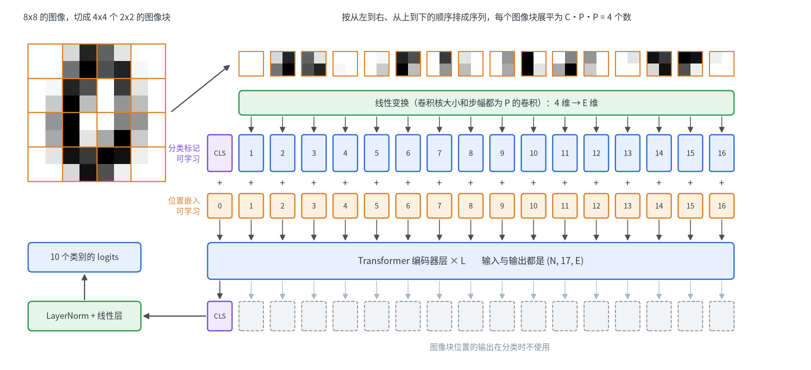
Vision Transformer(ViT)把图像切成固定大小的图像块,把每个图像块当作序列中的一个词元(token),之后直接使用标准的 Transformer 编码器。注意力、位置编码、编码器层的结构和参数量见PyTorch Transformer,卷积的输出尺寸与感受野见PyTorch CNN,这里只整理图像特有的部分:图像怎样变成序列、序列怎样变成分类结果,以及这种做法与卷积网络相比的代价
从图像到序列
| 符号 | 含义 | ViT-B/16 中的取值 |
|---|---|---|
| $C$ | 图像的通道数 | 3 |
| $P$ | 图像块的边长,patch_size | 16 |
| $G$ | 每条边上的图像块个数,图像边长除以$P$ | 14 |
| $E$ | 词元的向量维度 | 768 |
| $L$ | 序列长度,图像块个数加上一个分类标记 | 197 |
图像块嵌入
图像块嵌入做两件事:把图像切成互不重叠的$P \times P$小块,再用同一个线性层把每一块的$C \cdot P \cdot P$个像素值变成$E$维的向量。这两步等价于一个卷积核大小和步幅都为$P$的卷积:卷积核每次正好盖住一个图像块,并且不同的图像块共用同一组权重
1
2
3
4
5
6
7
8
9
10
11
12
13
14
15
16
17
18
19
20
21
22
23
24
25
26
27
28
29
30
31
32
33
34
import torch
import torch.nn.functional as F
from torch import nn

torch.manual_seed(0)
x = torch.randn(2, 3, 224, 224)
P, E = 16, 768

# 写法一:手动切块。先把高和宽各切成14段,再把每一块的像素展平
n, c, h, w = x.shape
patches = x.reshape(n, c, h // P, P, w // P, P)   # (2, 3, 14, 16, 14, 16)
patches = patches.permute(0, 2, 4, 1, 3, 5)       # (2, 14, 14, 3, 16, 16)
patches = patches.reshape(n, -1, c * P * P)       # (2, 196, 768)
print(patches.shape)

# F.unfold做的是同一件事,结果的形状为(N, C*P*P, 块数)
unfolded = F.unfold(x, kernel_size=P, stride=P).transpose(1, 2)
print(torch.equal(patches, unfolded))             # True

# 写法二:卷积核大小和步幅都等于P的卷积
conv = nn.Conv2d(c, E, kernel_size=P, stride=P)
tokens_conv = conv(x).flatten(2).transpose(1, 2)  # (2, 768, 14, 14) -> (2, 196, 768)

# 把卷积的权重(E, C, P, P)展平成(E, C*P*P),复制给线性层
linear = nn.Linear(c * P * P, E)
with torch.no_grad():
    linear.weight.copy_(conv.weight.reshape(E, -1))
    linear.bias.copy_(conv.bias)
tokens_linear = linear(patches)

print(tokens_conv.shape, tokens_linear.shape)
print(torch.allclose(tokens_conv, tokens_linear, atol=1e-5))  # True
print((tokens_conv - tokens_linear).abs().max().item())
print(sum(p.numel() for p in conv.parameters()), c * P * P * E + E)
1
2
3
4
5
6
torch.Size([2, 196, 768])
True
torch.Size([2, 196, 768]) torch.Size([2, 196, 768])
True
3.2186508178710938e-06
590592 590592
- 两种写法的结果只相差浮点数的舍入误差,参数量也相同,都是$C P^2 E + E$。实际代码中都用卷积,写法最短,速度也更快
- 这里图像块展平后恰好也是 768 维,只是因为$3 \times 16 \times 16 = 768$,与$E$没有必然关系
- 展平时各维的顺序是通道、行、列,与卷积权重
(E, C, P, P)展平的顺序一致,所以权重可以直接复制。permute的顺序写错时形状仍然正确,但每个图像块里的像素被打乱
词元数量
序列长度只由图像大小和图像块大小决定,与通道数和$E$无关
\[L = \frac{H}{P} \times \frac{W}{P} + 1\]| 图像大小 | 图像块大小 | 图像块个数 | 序列长度 $L$ |
|---|---|---|---|
| 224 | 32 | 7 × 7 | 50 |
| 224 | 16 | 14 × 14 | 197 |
| 224 | 14 | 16 × 16 | 257 |
| 384 | 16 | 24 × 24 | 577 |
| 1024 | 16 | 64 × 64 | 4097 |
图像块越小,每个词元保留的细节越多,但序列越长:图像块边长减半,序列长度变为 4 倍。模型名称中斜线后面的数字就是图像块大小,ViT-B/16 表示 Base 规模、图像块为 16 × 16
分类标记与位置嵌入
| 部分 | 形状 | 作用 |
|---|---|---|
| 分类标记 | (1, 1, E) | 一个可学习的向量,拼在序列最前面。它不对应任何图像块,经过各层注意力后汇集了所有图像块的信息,最后只用它的输出做分类 |
| 位置嵌入 | (1, L, E) | 每个位置一个可学习的向量,与词元相加。图像块展平成序列后,原来的行列关系只能靠它提供 |
- 分类标记对一个批次中的所有图像是同一个向量,前向传播时用
expand复制到批大小 - 位置嵌入是一维的编号,模型事先并不知道 14 × 14 的网格中第 1 个和第 15 个图像块上下相邻,这种二维关系要从数据中学出来
- 位置嵌入的长度在创建模型时就固定了,这是 ViT 不能直接处理其他分辨率的原因,处理方法见后面的改变输入分辨率
一个小型 ViT
下面的模型用于 8 × 8 的单通道图像,图像块大小为 2,共 16 个图像块。编码器层是手写的前归一化结构,目的是把注意力权重保留下来供后面查看。保存为vit.py,后面的代码会导入它
1
2
3
4
5
6
7
8
9
10
11
12
13
14
15
16
17
18
19
20
21
22
23
24
25
26
27
28
29
30
31
32
33
34
35
36
37
38
39
40
41
42
43
44
45
46
47
48
49
50
51
52
53
54
55
56
57
58
59
60
import torch
from torch import nn


class Block(nn.Module):
    """前归一化的编码器层,与nn.TransformerEncoderLayer(norm_first=True, activation="gelu")的结构相同"""

    def __init__(self, dim, heads, mlp_dim):
        super().__init__()
        self.norm1 = nn.LayerNorm(dim)
        self.attention = nn.MultiheadAttention(dim, heads, batch_first=True)
        self.norm2 = nn.LayerNorm(dim)
        self.mlp = nn.Sequential(nn.Linear(dim, mlp_dim), nn.GELU(), nn.Linear(mlp_dim, dim))
        self.weights = None                                    # 最近一次前向传播的注意力权重

    def forward(self, x):
        y = self.norm1(x)
        y, self.weights = self.attention(y, y, y, average_attn_weights=False)  # 权重: (N, H, L, L)
        x = x + y
        return x + self.mlp(self.norm2(x))


class ViT(nn.Module):
    def __init__(self, image_size=8, patch_size=2, in_channels=1, num_classes=10,
                 dim=64, depth=2, heads=4, mlp_dim=128, use_position=True):
        super().__init__()
        self.grid = image_size // patch_size                   # 每条边上的图像块个数
        self.patch_embedding = nn.Conv2d(in_channels, dim, kernel_size=patch_size, stride=patch_size)
        self.cls_token = nn.Parameter(torch.zeros(1, 1, dim))
        # use_position=False时位置嵌入保持为0并且不训练,只用于后面的对比实验
        self.position_embedding = nn.Parameter(torch.zeros(1, self.grid ** 2 + 1, dim), requires_grad=use_position)
        if use_position:
            nn.init.trunc_normal_(self.position_embedding, std=0.02)
        self.blocks = nn.ModuleList(Block(dim, heads, mlp_dim) for _ in range(depth))
        self.norm = nn.LayerNorm(dim)
        self.head = nn.Linear(dim, num_classes)

    def forward(self, x):
        x = self.patch_embedding(x)                            # (N, E, G, G)
        x = x.flatten(2).transpose(1, 2)                       # (N, G*G, E)
        cls_token = self.cls_token.expand(x.size(0), -1, -1)   # (N, 1, E)
        x = torch.cat([cls_token, x], dim=1)                   # (N, G*G + 1, E)
        x = x + self.position_embedding
        for block in self.blocks:
            x = block(x)
        x = self.norm(x)
        return self.head(x[:, 0])                              # 只取分类标记的输出


if __name__ == "__main__":
    model = ViT()
    print(model(torch.randn(5, 1, 8, 8)).shape)                # torch.Size([5, 10])
    print(model.blocks[-1].weights.shape)                      # torch.Size([5, 4, 17, 17])
    print(sum(p.numel() for p in model.parameters()))          # 69194

    def count(module):
        return sum(p.numel() for p in module.parameters())

    builtin = nn.TransformerEncoderLayer(64, 4, 128, activation="gelu", batch_first=True, norm_first=True)
    print(count(model.blocks[0]), count(builtin))              # 33472 33472
1
2
3
4
torch.Size([5, 10])
torch.Size([5, 4, 17, 17])
69194
33472 33472
前向传播中各步的形状如下,括号内是这个小模型的取值
| 步骤 | 输出形状 | 说明 |
|---|---|---|
| 输入图像 | (N, C, H, W) = (5, 1, 8, 8) | |
| 图像块嵌入的卷积 | (N, E, G, G) = (5, 64, 4, 4) | 每个空间位置对应一个图像块 |
flatten(2) | (N, E, G·G) = (5, 64, 16) | 把两个空间维合并 |
transpose(1, 2) | (N, G·G, E) = (5, 16, 64) | 换成 Transformer 使用的 (N, L, E) |
| 拼接分类标记 | (N, G·G + 1, E) = (5, 17, 64) | 分类标记在第 0 个位置 |
| 加位置嵌入 | (5, 17, 64) | 形状为 (1, 17, 64),对批次维广播 |
| 每个编码器层 | (5, 17, 64) | 形状不变,注意力权重为 (N, H, L, L) |
LayerNorm | (5, 17, 64) | 前归一化时最后一层的输出没有归一化,在这里补上 |
| 取第 0 个位置 | (N, E) = (5, 64) | 分类标记的输出 |
| 分类头 | (N, K) = (5, 10) |
- 整个模型里只有图像块嵌入和位置嵌入与图像有关,中间的编码器层与处理文本时完全相同
- 手写的
Block与自带的nn.TransformerEncoderLayer参数量相同。只需要输出、不需要注意力权重时可以直接用自带的层
参数量
计算公式
| 部分 | 参数量 | 说明 |
|---|---|---|
| 图像块嵌入 | $C P^2 E + E$ | 一个卷积 |
| 分类标记 | $E$ | |
| 位置嵌入 | $L E$ | 与分辨率有关的唯一一项 |
| 一个编码器层 | $(4E^2 + 4E) + (2EM + M + E) + 4E$ | 注意力、前馈网络、两个LayerNorm,$M$为前馈网络的中间维度 |
| 最后的归一化 | $2E$ | |
| 分类头 | $E K + K$ | $K$为类别数 |
用公式计算 ViT-B/16 的参数量,并与torchvision中的模型对照。只看结构不需要下载权重,weights=None即可
1
2
3
4
5
6
7
8
9
10
11
12
13
14
15
16
17
18
19
20
21
22
23
24
25
26
27
28
29
30
31
32
33
34
35
36
37
38
39
40
41
42
43
44
45
import torch
from torchvision.models import vit_b_16


def vit_params(image_size, patch_size, dim, depth, mlp_dim, num_classes, channels=3):
    tokens = (image_size // patch_size) ** 2 + 1
    patch_embedding = channels * patch_size ** 2 * dim + dim
    block = (4 * dim ** 2 + 4 * dim) + (2 * dim * mlp_dim + mlp_dim + dim) + 2 * 2 * dim
    return {
        "patch_embedding": patch_embedding,
        "cls_token": dim,
        "position_embedding": tokens * dim,
        "blocks": depth * block,
        "norm": 2 * dim,
        "head": dim * num_classes + num_classes,
    }


# 上一节的小模型
print(sum(vit_params(image_size=8, patch_size=2, dim=64, depth=2, mlp_dim=128, num_classes=10, channels=1).values()))

# ViT-B/16
parts = vit_params(image_size=224, patch_size=16, dim=768, depth=12, mlp_dim=3072, num_classes=1000)
for name, value in parts.items():
    print(f"{name:20s}{value:>11,}")
print(f"{'total':20s}{sum(parts.values()):>11,}")

model = vit_b_16(weights=None).eval()
print(sum(p.numel() for p in model.parameters()))  # 86567656
print(model.conv_proj)
print(model.class_token.shape, model.encoder.pos_embedding.shape)
print(len(model.encoder.layers), model.heads.head)

# 逐步执行前向传播,查看每一步的形状
x = torch.randn(2, 3, 224, 224)
with torch.no_grad():
    tokens = model._process_input(x)                       # 切块并做线性变换
    print(tokens.shape)                                    # torch.Size([2, 196, 768])
    tokens = torch.cat([model.class_token.expand(2, -1, -1), tokens], dim=1)
    print(tokens.shape)                                    # torch.Size([2, 197, 768])
    encoded = model.encoder(tokens)                        # 加位置嵌入、12个编码器层、LayerNorm
    print(encoded.shape)                                   # torch.Size([2, 197, 768])
    logits = model.heads(encoded[:, 0])
    print(logits.shape)                                    # torch.Size([2, 1000])
    print(torch.allclose(logits, model(x), atol=1e-5))     # True
1
2
3
4
5
6
7
8
9
10
11
12
13
14
15
16
17
69194
patch_embedding         590,592
cls_token                   768
position_embedding      151,296
blocks               85,054,464
norm                      1,536
head                    769,000
total                86,567,656
86567656
Conv2d(3, 768, kernel_size=(16, 16), stride=(16, 16))
torch.Size([1, 1, 768]) torch.Size([1, 197, 768])
12 Linear(in_features=768, out_features=1000, bias=True)
torch.Size([2, 196, 768])
torch.Size([2, 197, 768])
torch.Size([2, 197, 768])
torch.Size([2, 1000])
True
- 公式的结果与两个模型都完全一致:小模型 69,194,ViT-B/16 为 86,567,656。其中 98% 的参数在编码器层里,图像块嵌入和位置嵌入加起来不到 1%
torchvision的实现与上面的小模型步骤相同:conv_proj是图像块嵌入,class_token是分类标记,位置嵌入放在encoder里,分类头是heads.head,替换分类头的写法见PyTorch Fine-Tuning
torchvision 中的规格
1
2
3
4
5
6
7
8
from torchvision.models import vit_b_16, vit_b_32, vit_h_14, vit_l_16, vit_l_32

for make in [vit_b_32, vit_b_16, vit_l_32, vit_l_16, vit_h_14]:
    model = make(weights=None)
    layer = model.encoder.layers[0]
    print(f"{make.__name__:9s} patch {model.patch_size:2d}  tokens {model.seq_length:3d}  dim {model.hidden_dim:4d}"
          f"  depth {len(model.encoder.layers):2d}  heads {layer.self_attention.num_heads:2d}"
          f"  mlp {layer.mlp[0].out_features}  params {sum(p.numel() for p in model.parameters()):>11,}")
1
2
3
4
5
vit_b_32  patch 32  tokens  50  dim  768  depth 12  heads 12  mlp 3072  params  88,224,232
vit_b_16  patch 16  tokens 197  dim  768  depth 12  heads 12  mlp 3072  params  86,567,656
vit_l_32  patch 32  tokens  50  dim 1024  depth 24  heads 16  mlp 4096  params 306,535,400
vit_l_16  patch 16  tokens 197  dim 1024  depth 24  heads 16  mlp 4096  params 304,326,632
vit_h_14  patch 14  tokens 257  dim 1280  depth 32  heads 16  mlp 5120  params 632,045,800
- 图像块从 16 增大到 32,参数量反而略有增加:图像块嵌入的卷积核变大了,而编码器层的参数量与序列长度无关
- 图像块大小影响的是计算量:
vit_b_32的序列长度只有vit_b_16的四分之一,计算量也相应减少,代价是每个词元对应的区域更粗
与 CNN 的对比实验
实验设置
在sklearn自带的 8 × 8 手写数字上,比较上面的小型 ViT 和一个参数量相近的 CNN。1797 张图像中固定取 497 张作测试集,从其余 1300 张中抽取 50 到 1300 张作训练集,观察两种模型对数据量的依赖
| 项目 | 设置 |
|---|---|
| ViT | 上一节的模型,69,194 个参数;另有一个去掉位置嵌入的版本 |
| CNN | 3 个 3 × 3 卷积加BatchNorm,中间一次池化,全局平均池化后接线性层,56,714 个参数 |
| 训练 | 三种模型的设置完全相同:AdamW,学习率 1e-3,权重衰减 0.05,批大小 64,共 600 步,学习率先升后降,不做数据增强 |
| 重复 | 每种设置用 3 个随机种子,种子同时决定初始权重和抽到的训练图像 |
1
2
3
4
5
6
7
8
9
10
11
12
13
14
15
16
17
18
19
20
21
22
23
24
25
26
27
28
29
30
31
32
33
34
35
36
37
38
39
40
41
42
43
44
45
46
47
48
49
50
51
52
53
54
55
56
57
58
59
60
61
62
63
64
65
66
import json

import torch
import torch.nn.functional as F
from sklearn.datasets import load_digits
from torch import nn

from vit import ViT


def make_cnn():
    return nn.Sequential(
        nn.Conv2d(1, 32, 3, padding=1), nn.BatchNorm2d(32), nn.ReLU(),
        nn.Conv2d(32, 64, 3, padding=1), nn.BatchNorm2d(64), nn.ReLU(), nn.MaxPool2d(2),
        nn.Conv2d(64, 64, 3, padding=1), nn.BatchNorm2d(64), nn.ReLU(),
        nn.AdaptiveAvgPool2d(1), nn.Flatten(), nn.Linear(64, 10))


# 8x8的手写数字,共1797张:固定取497张作测试集,其余1300张中抽取不同数量作训练集
digits = load_digits()
images = torch.tensor(digits.images, dtype=torch.float32).unsqueeze(1) / 16   # (1797, 1, 8, 8)
labels = torch.tensor(digits.target)
order = torch.randperm(len(images), generator=torch.Generator().manual_seed(0))
test_idx, pool = order[:497], order[497:]


def train(make_model, size, seed, steps=600, batch_size=64, lr=1e-3):
    """三种模型使用完全相同的设置:AdamW、600步、学习率先升后降"""
    torch.manual_seed(seed)
    model = make_model()
    train_idx = pool[torch.randperm(len(pool))[:size]]
    optimizer = torch.optim.AdamW(model.parameters(), lr=lr, weight_decay=0.05)
    scheduler = torch.optim.lr_scheduler.OneCycleLR(optimizer, max_lr=lr, total_steps=steps, pct_start=0.1)
    model.train()
    for _ in range(steps):
        batch = train_idx[torch.randint(0, size, (min(batch_size, size),))]
        loss = F.cross_entropy(model(images[batch]), labels[batch])
        optimizer.zero_grad()
        loss.backward()
        optimizer.step()
        scheduler.step()
    model.eval()
    with torch.no_grad():
        accuracy = (model(images[test_idx]).argmax(dim=1) == labels[test_idx]).float().mean().item()
    return model, accuracy


models = {"ViT": ViT, "ViT 无位置嵌入": lambda: ViT(use_position=False), "CNN": make_cnn}
for name, make_model in models.items():
    print(f"{name} 参数量 {sum(p.numel() for p in make_model().parameters() if p.requires_grad):,}")

sizes = [50, 100, 200, 400, 800, 1300]
results = {name: [] for name in models}
for size in sizes:
    line = f"{size:>5d}"
    for name, make_model in models.items():
        accuracies = [train(make_model, size, seed)[1] for seed in range(3)]   # 3个随机种子
        results[name].append(accuracies)
        line += f"   {name} {sum(accuracies) / 3:.3f} ({min(accuracies):.3f} ~ {max(accuracies):.3f})"
    print(line)
json.dump({"sizes": sizes, "accuracy": results}, open("data_size.json", "w"), ensure_ascii=False)

# 保存一个用全部1300张训练的ViT,后面查看注意力时使用
model, accuracy = train(ViT, 1300, seed=0)
torch.save(model.state_dict(), "vit_digits.pt")
print(f"{accuracy:.3f}")
1
2
3
4
5
6
7
8
9
10
ViT 参数量 69,194
ViT 无位置嵌入 参数量 68,106
CNN 参数量 56,714
   50   ViT 0.565 (0.513 ~ 0.622)   ViT 无位置嵌入 0.391 (0.388 ~ 0.394)   CNN 0.871 (0.851 ~ 0.885)
  100   ViT 0.700 (0.680 ~ 0.718)   ViT 无位置嵌入 0.447 (0.419 ~ 0.473)   CNN 0.923 (0.909 ~ 0.934)
  200   ViT 0.826 (0.803 ~ 0.867)   ViT 无位置嵌入 0.565 (0.531 ~ 0.584)   CNN 0.967 (0.960 ~ 0.974)
  400   ViT 0.890 (0.869 ~ 0.909)   ViT 无位置嵌入 0.670 (0.650 ~ 0.696)   CNN 0.980 (0.976 ~ 0.986)
  800   ViT 0.941 (0.934 ~ 0.948)   ViT 无位置嵌入 0.736 (0.732 ~ 0.738)   CNN 0.989 (0.984 ~ 0.992)
 1300   ViT 0.947 (0.946 ~ 0.948)   ViT 无位置嵌入 0.766 (0.761 ~ 0.769)   CNN 0.995 (0.992 ~ 0.998)
0.946
结果
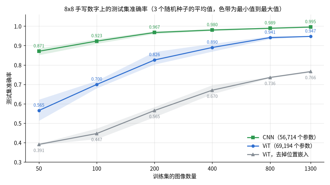
- CNN 在每个数据量下都更好,数据越少差距越大:50 张时 ViT 为 0.565、CNN 为 0.871,相差 0.306;1300 张时为 0.947 和 0.995,差距缩小到 0.048
- 换一个角度看,CNN 用 100 张图像达到 0.923,ViT 要用到 800 张才超过这个水平
- 去掉位置嵌入后,1300 张时也只有 0.766。注意力本身不区分顺序,没有位置嵌入时模型看到的只是一组无序的图像块,只能靠每个图像块里的内容分类
- 把
steps改为 2000 重新运行,1300 张时 ViT 升到 0.965、CNN 仍为 0.995,50 张时 ViT 为 0.542、CNN 为 0.875。训练更久能缩小数据充足时的差距,数据少时没有帮助 - 这个实验规模很小,没有数据增强,两种模型也都没有单独调参,结论只在这个范围内成立:ViT 的准确率随数据量上升得更快,但直到用完全部数据也没有追上 CNN。ViT 超过 CNN 的结果出现在用远大于 ImageNet-1K 的数据集预训练之后,这里没有验证
归纳偏置
差距来自两种结构对图像所做的假设不同。CNN 把图像的性质写进了结构里,ViT 把它们留给数据
| 性质 | CNN | ViT |
|---|---|---|
| 局部性 | 卷积核只连接相邻的像素 | 只有图像块内部是局部的,图像块之间谁离谁近要从数据中学 |
| 平移 | 同一个卷积核滑过所有位置,权重共享 | 图像块嵌入共享权重,但每个位置的位置嵌入各不相同 |
| 二维结构 | 特征图始终是二维的 | 展平成一维序列,行列关系完全依赖学到的位置嵌入 |
| 感受野 | 随层数逐渐扩大 | 第一层的注意力就能看到整张图像 |
假设越少,模型能表示的函数越多,但需要更多的数据才能把这些本来可以写进结构的规律学出来。数据少时让 ViT 可用的办法主要有三种:使用在大数据集上预训练的权重再微调,加强数据增强和正则化,或者在结构中加回一部分卷积的性质,见最后一节的表格
改变输入分辨率
位置嵌入的插值
ViT 中与分辨率有关的参数只有位置嵌入。换一个分辨率时,把图像块的位置嵌入还原成$G \times G$的二维网格,像缩放图像一样插值到新的网格大小,分类标记的那一个保持不变
1
2
3
4
5
6
7
8
9
10
11
12
13
14
15
16
17
18
19
20
21
22
23
24
25
26
27
28
29
30
31
32
33
34
35
36
37
38
39
40
import torch
import torch.nn.functional as F
from torchvision.models import vit_b_16
from torchvision.models.vision_transformer import interpolate_embeddings


def resize_position_embedding(position, new_grid):
    """position: (1, 1 + G*G, E),第0个是分类标记的位置嵌入,不参与插值"""
    cls_position, patch_position = position[:, :1], position[:, 1:]
    old_grid = int(patch_position.size(1) ** 0.5)
    dim = position.size(-1)
    grid = patch_position.reshape(1, old_grid, old_grid, dim).permute(0, 3, 1, 2)   # (1, E, G, G)
    grid = F.interpolate(grid, size=(new_grid, new_grid), mode="bicubic", align_corners=True)
    patch_position = grid.permute(0, 2, 3, 1).reshape(1, new_grid * new_grid, dim)
    return torch.cat([cls_position, patch_position], dim=1)


torch.manual_seed(0)
model = vit_b_16(weights=None).eval()                 # 代替一个在224x224上训练好的模型
state = model.state_dict()
print(state["encoder.pos_embedding"].shape)           # torch.Size([1, 197, 768])

new_position = resize_position_embedding(state["encoder.pos_embedding"], new_grid=384 // 16)
print(new_position.shape)                             # torch.Size([1, 577, 768])

# 与torchvision自带的函数结果一致
reference = interpolate_embeddings(image_size=384, patch_size=16, model_state=state)
print(torch.allclose(new_position, reference["encoder.pos_embedding"], atol=1e-6))  # True

# 其余权重的形状都与分辨率无关,换掉位置嵌入就能加载到384x384的模型中
state["encoder.pos_embedding"] = new_position
large = vit_b_16(weights=None, image_size=384).eval()
print(large.load_state_dict(state))                   # <All keys matched successfully>
with torch.no_grad():
    print(large(torch.randn(1, 3, 384, 384)).shape)   # torch.Size([1, 1000])

try:
    model(torch.randn(1, 3, 384, 384))
except AssertionError as e:
    print(e)
1
2
3
4
5
6
torch.Size([1, 197, 768])
torch.Size([1, 577, 768])
True
<All keys matched successfully>
torch.Size([1, 1000])
Wrong image height! Expected 224 but got 384!
torchvision的 ViT 在前向传播时检查输入大小,与创建时的image_size不一致就报错,不会自动插值。要换分辨率,需要按新的image_size创建模型,再加载插值后的权重- 插值只保证形状能对上。图像块大小不变而分辨率提高后,每个图像块覆盖的内容变小了,与预训练时不同,通常要在新的分辨率上再微调:常见的用法就是在较低的分辨率上预训练,再在较高的分辨率上微调
- 这里的模型是随机初始化的,只验证了形状和加载过程,没有验证插值后的准确率
分辨率与计算量
序列长度与图像边长的平方成正比,注意力权重矩阵的大小又与序列长度的平方成正比,所以注意力权重的元素个数与边长的四次方成正比。下面在一台 CPU 为 Intel Core Ultra 9 285K、GPU 为 GeForce RTX 5090 D(32 GB 显存)、内存为 64 GB 的机器上,用 GPU 测量 ViT-B/16 在不同分辨率下推理的耗时和显存,批大小为 2,同时单独测量一层注意力
1
2
3
4
5
6
7
8
9
10
11
12
13
14
15
16
17
18
19
20
21
22
23
24
25
26
27
28
29
30
31
32
33
34
35
36
37
38
39
40
41
42
43
44
import json
import time

import torch
from torch import nn
from torchvision.models import vit_b_16

assert torch.cuda.is_available(), '这个例子需要GPU'


@torch.no_grad()
def measure(function, repeat=5):
    """返回平均耗时(毫秒)和运行期间额外占用的显存峰值(MB)"""
    function()                                    # 预热
    torch.cuda.synchronize()
    torch.cuda.reset_peak_memory_stats()
    before = torch.cuda.memory_allocated()        # 模型和输入本身占用的显存
    start = time.perf_counter()
    for _ in range(repeat):
        function()
    torch.cuda.synchronize()
    ms = (time.perf_counter() - start) / repeat * 1000
    return ms, (torch.cuda.max_memory_allocated() - before) / 2 ** 20


attention = nn.MultiheadAttention(768, 12, batch_first=True).eval().cuda()
results = []
for image_size in [224, 384, 512, 768, 1024]:
    tokens = (image_size // 16) ** 2 + 1
    model = vit_b_16(weights=None, image_size=image_size).eval().cuda()
    x = torch.randn(2, 3, image_size, image_size, device="cuda")
    model_ms, model_mb = measure(lambda: model(x))
    # 单独一层注意力:不返回权重,以及返回每个头的权重
    y = torch.randn(2, tokens, 768, device="cuda")
    fast_ms, fast_mb = measure(lambda: attention(y, y, y, need_weights=False))
    full_ms, full_mb = measure(lambda: attention(y, y, y, average_attn_weights=False))

    print(f"{image_size:>5d} {tokens:>5d} | {model_ms:6.1f} ms {model_mb:5.0f} MB"
          f" | {fast_ms:5.2f} ms {fast_mb:5.0f} MB | {full_ms:6.2f} ms {full_mb:5.0f} MB")
    results.append({"image_size": image_size, "tokens": tokens, "model_ms": model_ms, "model_mb": model_mb,
                    "fast_ms": fast_ms, "fast_mb": fast_mb, "full_ms": full_ms, "full_mb": full_mb})
    del model, x, y
    torch.cuda.empty_cache()
json.dump(results, open("cost.json", "w"))
1
2
3
4
5
  224   197 |    3.5 ms    19 MB |  0.11 ms     8 MB |   0.14 ms    39 MB
  384   577 |    7.6 ms    44 MB |  0.33 ms    18 MB |   0.29 ms    73 MB
  512  1025 |   11.9 ms    78 MB |  0.51 ms    31 MB |   0.61 ms   146 MB
  768  2305 |   32.6 ms   177 MB |  1.65 ms    70 MB |   2.30 ms   559 MB
 1024  4097 |   76.3 ms   312 MB |  4.28 ms   121 MB |   6.41 ms  1658 MB
各列依次为图像边长、序列长度,整个模型的耗时和显存,一层注意力不返回权重时的耗时和显存,一层注意力返回每个头的权重时的耗时和显存。耗时每次运行略有波动,这里是多次运行中的典型值
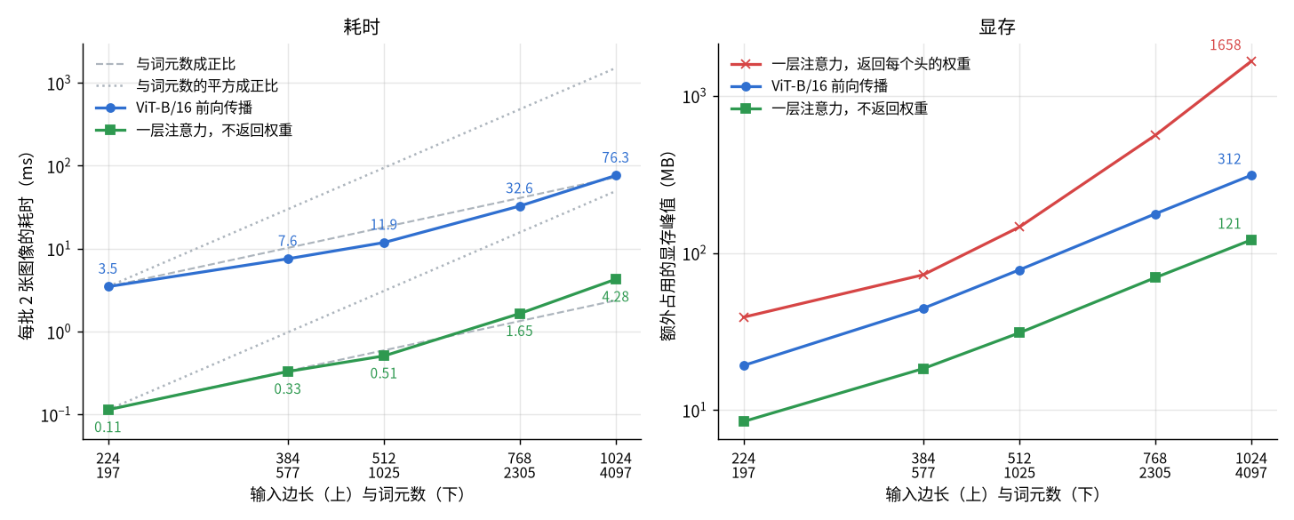
- 返回权重时,显存明显按平方增长:序列长度从 2305 到 4097 增加到 1.78 倍,显存从 559 MB 到 1658 MB,为 2.97 倍。4097 个词元、12 个头、批大小 2 的权重矩阵本身就有$2 \times 12 \times 4097^2$个元素,约 1537 MB
- 不返回权重时,
nn.MultiheadAttention在推理时使用F.scaled_dot_product_attention,不保存完整的权重矩阵,显存基本与序列长度成正比。torchvision的 ViT 内部就是这样调用的,所以整个模型的显存也接近线性 - 整个模型的耗时在这个范围内大致与序列长度成正比:序列长度变为 20.8 倍,耗时变为 21.9 倍。序列短时每一层的计算量很小,GPU 没有被占满,而且前馈网络等与序列长度成正比的部分占了大头;平方项到序列很长时才显现,从 2305 到 4097,耗时变为 2.34 倍,已经超过了序列长度的 1.78 倍
- 即使只是线性增长,代价也不小:边长从 224 增加到 1024,耗时和显存都变为原来的 16 到 22 倍。检测、分割这类需要高分辨率的任务因此很少直接使用全局注意力的 ViT,而是限制注意力的范围,见最后一节
分类标记关注的位置
分类只使用分类标记的输出,所以最后一层中分类标记作为查询时的注意力权重,表示分类结果主要取自哪些图像块。前面的Block把权重保存在了weights中,下面用对比实验中保存的模型查看
1
2
3
4
5
6
7
8
9
10
11
12
13
14
15
16
17
18
19
20
21
22
23
24
25
26
27
28
29
30
31
32
33
34
35
36
37
import numpy as np
import torch
from sklearn.datasets import load_digits

from vit import ViT

digits = load_digits()
images = torch.tensor(digits.images, dtype=torch.float32).unsqueeze(1) / 16
labels = torch.tensor(digits.target)
order = torch.randperm(len(images), generator=torch.Generator().manual_seed(0))
test_idx = order[:497]                                  # 与训练时相同的测试集

model = ViT()
model.load_state_dict(torch.load("vit_digits.pt"))
model.eval()

x, y = images[test_idx], labels[test_idx]
with torch.no_grad():
    predictions = model(x).argmax(dim=1)
weights = model.blocks[-1].weights                      # 最后一层的注意力权重
print(weights.shape)                                    # torch.Size([497, 4, 17, 17])
print(torch.allclose(weights.sum(dim=-1), torch.ones(497, 4, 17)))  # True,每一行之和为1

# 第0行是分类标记作为查询时的权重:第0列是它对自己的关注,其余16列对应16个图像块
cls_attention = weights[:, :, 0, 1:].mean(dim=1)        # 对4个头取平均,(497, 16)
maps = cls_attention.reshape(-1, model.grid, model.grid)  # (497, 4, 4)
print(maps.shape)
print(f"{weights[:, :, 0, 0].mean().item():.3f} {cls_attention.sum(dim=1).mean().item():.3f}")
print(f"{(predictions == y).float().mean().item():.3f}")

torch.set_printoptions(precision=2, sci_mode=False)
first = (y == 0).nonzero()[0].item()                    # 测试集中第一张数字0
print(maps[first])
# 每个类别取一张,保存图像和对应的注意力图
chosen = [(y == k).nonzero()[0].item() for k in range(10)]
np.savez("attention.npz", images=x[chosen, 0].numpy(), maps=maps[chosen].numpy(),
         labels=y[chosen].numpy(), predictions=predictions[chosen].numpy())
1
2
3
4
5
6
7
8
9
torch.Size([497, 4, 17, 17])
True
torch.Size([497, 4, 4])
0.177 0.823
0.946
tensor([[0.02, 0.09, 0.04, 0.03],
        [0.02, 0.01, 0.41, 0.02],
        [0.04, 0.02, 0.24, 0.01],
        [0.01, 0.01, 0.01, 0.01]])
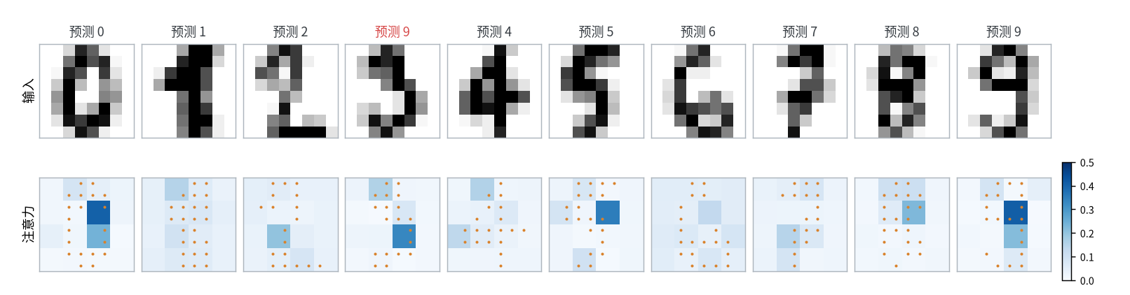
- 权重的每一行之和为 1。分类标记平均把 0.177 的权重留给自己,其余 0.823 分给 16 个图像块
- 权重并不是均匀分布的。上面打印的是图中数字 0 的注意力,第 2、3 行第 3 列的两个图像块分别为 0.41 和 0.24,对应右侧笔画与中间空洞相接的地方
- 集中的程度因数字而异:图中的 0、5、9 最大的一个图像块占 0.35 到 0.41,而 1、4、6、7 最大的也只有 0.13 到 0.16,分散在多个图像块上
- 图中的数字 3 被误判为 9,注意力最大的图像块在第 3 行第 3 列,占 0.33
- 这里的图像块只有 4 × 4 个,注意力图很粗糙;在 ViT-B/16 上同样的做法得到 14 × 14 的图,放大后叠在原图上查看。注意力权重只说明最后一层从哪些位置取信息。前面的层已经在图像块之间交换过信息,某个位置的输出不再只代表它自己那一块图像,所以这种图只能作为参考,不能当作模型判断依据的完整解释
- 要查看每个头各自的权重,去掉
mean(dim=1)即可;nn.TransformerEncoderLayer内部不返回权重,这也是这里手写Block的原因
变体与相关结构
| 结构 | 与 ViT 的区别 | 解决的问题 |
|---|---|---|
| DeiT | 结构不变,改的是训练方法:更强的数据增强和正则化,并用一个 CNN 作教师做蒸馏 | 只用 ImageNet-1K 也能把 ViT 训练好 |
| 混合结构 | 先用几层卷积提取特征图,再把特征图切块送入 Transformer | 用卷积补上局部性,数据较少时更容易训练 |
| Swin Transformer | 注意力只在局部窗口内计算,窗口逐层错开;每个阶段合并相邻的图像块,分辨率逐级减半 | 计算量与图像大小成正比,并提供多尺度特征 |
| 用 ViT 做检测、分割 | 不用分类标记,把图像块位置的输出还原成$G \times G$的特征图,交给检测头或分割头 | 让 ViT 作为密集预测任务的主干 |
| MAE | 结构不变,预训练时遮住大部分图像块,让模型重建被遮住的像素 | 不需要标注就能预训练 |
- 这一节没有做实验,只列出各个结构的出发点。
torchvision.models中有swin_t、swin_v2_t等 Swin 模型和vit_*系列,DeiT 等其他变体可以使用timm库 - 检测与分割的头见Object Detection和Image Segmentation