Object Detection
整理目标检测的基本组成:边界框格式、IoU、非极大值抑制、锚框、检测头输出的解码、损失函数、mAP 的计算,以及预训练检测器的使用和坐标映射
深度学习系列:第 17 篇,共 22 篇
用 PyTorch 从搭建模型、训练、调试到部署的一组笔记。按下面的顺序阅读,后面的文章会直接引用前面讲过的内容
目标检测要同时回答图像中有什么和在哪里:对每个目标输出一个边界框、一个类别和一个置信度分数。不同的检测模型结构差别很大,但边界框的表示、IoU、非极大值抑制、解码、损失函数和评价指标是通用的,torchvision.ops中有对应的实现
边界框的表示
边界框是与图像坐标轴平行的矩形,用 4 个数表示。图像坐标系的原点在左上角,$x$向右,$y$向下,与 OpenCV 一致
| 格式 | 4 个数的含义 | 常见的使用场合 |
|---|---|---|
xyxy | 左上角和右下角的坐标 | torchvision的模型和函数、Pascal VOC |
xywh | 左上角的坐标、宽度、高度 | COCO 标注文件、cv2.boundingRect的返回值 |
cxcywh | 中心点的坐标、宽度、高度 | YOLO 系列的标注和网络输出、DETR |
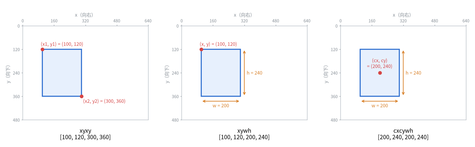
坐标还分为绝对坐标(以像素为单位)和归一化坐标(除以图像的宽度和高度,取值在 0 到 1 之间)。YOLO 的标注文件使用归一化的cxcywh,好处是图像缩放后标注不需要修改
torchvision.ops.box_convert在三种格式之间转换,输入的形状为 (N, 4)
1
2
3
4
5
6
7
8
9
10
11
12
13
14
15
16
17
18
import torch
from torchvision.ops import box_convert

# 640x480 图像上的一个框,左上角 (100, 120),右下角 (300, 360)
xyxy = torch.tensor([[100., 120., 300., 360.]])

xywh = box_convert(xyxy, in_fmt='xyxy', out_fmt='xywh')
cxcywh = box_convert(xyxy, in_fmt='xyxy', out_fmt='cxcywh')
print(xywh)    # tensor([[100., 120., 200., 240.]])
print(cxcywh)  # tensor([[200., 240., 200., 240.]])

# 归一化:x 除以图像宽度,y 除以图像高度
width, height = 640, 480
scale = torch.tensor([width, height, width, height])
print(cxcywh / scale)  # tensor([[0.3125, 0.5000, 0.3125, 0.5000]])

# 转换回来
print(box_convert(cxcywh, in_fmt='cxcywh', out_fmt='xyxy'))  # tensor([[100., 120., 300., 360.]])
torchvision.ops中计算 IoU、做非极大值抑制的函数都要求xyxy格式,并且不检查输入。 传入其他格式不会报错,只会得到错误的结果,从标注文件或其他框架拿到边界框后要先确认格式
IoU
计算方法
IoU(Intersection over Union,交并比)衡量两个框的重合程度,是两个框交集的面积与并集的面积之比,取值在 0 到 1 之间
\[IoU = \frac{\operatorname{area}(A \cap B)}{\operatorname{area}(A \cup B)}\]交集仍然是一个矩形:左上角取两个框左上角中较大的坐标,右下角取两个框右下角中较小的坐标。并集的面积等于两个框的面积之和减去交集的面积
1
2
3
4
5
6
7
8
9
10
11
12
13
14
15
16
17
18
19
20
21
22
23
24
25
26
27
28
29
30
31
32
33
34
import torch
from torchvision.ops import box_iou


def iou(boxes1, boxes2):
    """boxes1: (N, 4),boxes2: (M, 4),均为 xyxy 格式,返回 (N, M)"""
    area1 = (boxes1[:, 2] - boxes1[:, 0]) * (boxes1[:, 3] - boxes1[:, 1])
    area2 = (boxes2[:, 2] - boxes2[:, 0]) * (boxes2[:, 3] - boxes2[:, 1])

    # 交集的左上角取两个框左上角的较大值,右下角取较小值
    left_top = torch.max(boxes1[:, None, :2], boxes2[None, :, :2])      # (N, M, 2)
    right_bottom = torch.min(boxes1[:, None, 2:], boxes2[None, :, 2:])  # (N, M, 2)
    wh = (right_bottom - left_top).clamp(min=0)  # 不相交时宽或高为负,截断为 0
    inter = wh[..., 0] * wh[..., 1]

    return inter / (area1[:, None] + area2[None, :] - inter)


gt = torch.tensor([[100., 100., 300., 300.]])
pred = torch.tensor([
    [100., 100., 300., 300.],  # 完全重合
    [120., 120., 320., 320.],  # 偏移 20 像素
    [150., 150., 350., 350.],  # 偏移 50 像素
    [200., 200., 400., 400.],  # 偏移 100 像素
    [150., 150., 250., 250.],  # 在真实框内部
    [320., 100., 420., 300.],  # 不相交
])

print(iou(gt, pred))      # tensor([[1.0000, 0.6807, 0.3913, 0.1429, 0.2500, 0.0000]])
print(box_iou(gt, pred))  # tensor([[1.0000, 0.6807, 0.3913, 0.1429, 0.2500, 0.0000]])

# 格式传错不会报错:把 xywh 格式的框当作 xyxy 传入,框与自身的 IoU 都不是 1
xywh = torch.tensor([[100., 100., 50., 50.]])
print(box_iou(xywh, xywh))  # tensor([[0.]])
box_iou接收 (N, 4) 和 (M, 4) 两组框,返回 (N, M) 的矩阵,即每一对框的 IoU
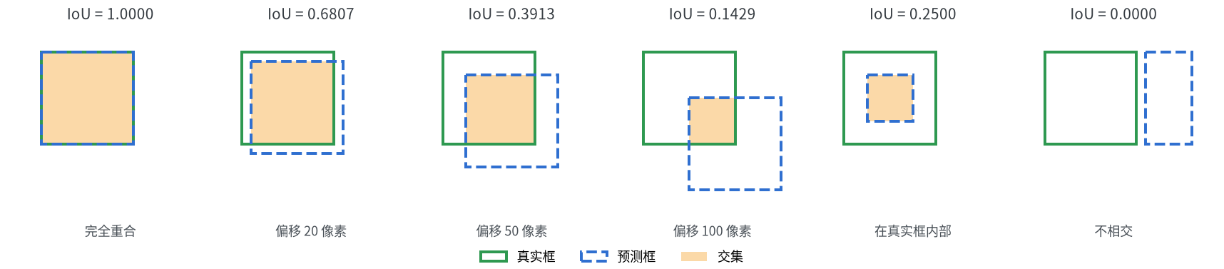
IoU 对位置偏差很敏感:边长 200 的框偏移 20 像素(边长的 10%),IoU 就降到 0.68;偏移 50 像素降到 0.39。评价时常用的阈值 0.5 并不宽松
GIoU、DIoU 与 CIoU
IoU 用作损失函数时有两个问题:两个框不相交时 IoU 恒为 0,无法反映相距多远;一个框包含另一个框时,无论小框在什么位置 IoU 都相同。下面三种改进在 IoU 的基础上减去一个惩罚项
| 名称 | 在 IoU 基础上减去的惩罚项 | torchvision.ops中的函数 |
|---|---|---|
| GIoU | 最小外接框中没有被两个框覆盖的面积所占的比例 | generalized_box_iou |
| DIoU | 两个框中心点距离的平方除以最小外接框对角线的平方 | distance_box_iou |
| CIoU | DIoU 的惩罚项,再加上宽高比不一致的惩罚 | complete_box_iou |
最小外接框是能同时包住两个框的最小矩形。三者的取值范围都从 IoU 的 0 到 1 扩展到了负数,两个框完全重合时都等于 1
1
2
3
4
5
6
7
8
9
10
11
12
13
14
15
import torch
from torchvision.ops import box_iou, generalized_box_iou, distance_box_iou, complete_box_iou

gt = torch.tensor([[100., 100., 300., 300.]])
pred = torch.tensor([
    [150., 150., 350., 350.],  # 部分重叠
    [320., 100., 420., 300.],  # 不相交,相距 20 像素
    [500., 100., 600., 300.],  # 不相交,相距 200 像素
    [150., 150., 250., 250.],  # 在真实框内部,居中
    [100., 100., 200., 200.],  # 在真实框内部,靠左上角
    [150., 175., 250., 225.],  # 在真实框内部,居中,宽高比不同
])

for name, fn in [('IoU', box_iou), ('GIoU', generalized_box_iou), ('DIoU', distance_box_iou), ('CIoU', complete_box_iou)]:
    print(f'{name:5s}', ' '.join(f'{v:8.4f}' for v in fn(gt, pred)[0].tolist()))
1
2
3
4
IoU     0.3913   0.0000   0.0000   0.2500   0.2500   0.1250
GIoU    0.3113  -0.0625  -0.4000   0.2500   0.2500   0.1250
DIoU    0.3513  -0.2029  -0.4224   0.2500   0.1875   0.1250
CIoU    0.3513  -0.2046  -0.4241   0.2500   0.1875   0.1231
- 第 2、3 列:两个不相交的框 IoU 都是 0,GIoU、DIoU、CIoU 则是相距越远数值越小
- 第 4、5 列:预测框在真实框内部时,居中和靠角落的 IoU 与 GIoU 相同,DIoU 能区分
- 第 6 列:中心重合但宽高比不同时,只有 CIoU 多了一项惩罚
非极大值抑制
计算方法
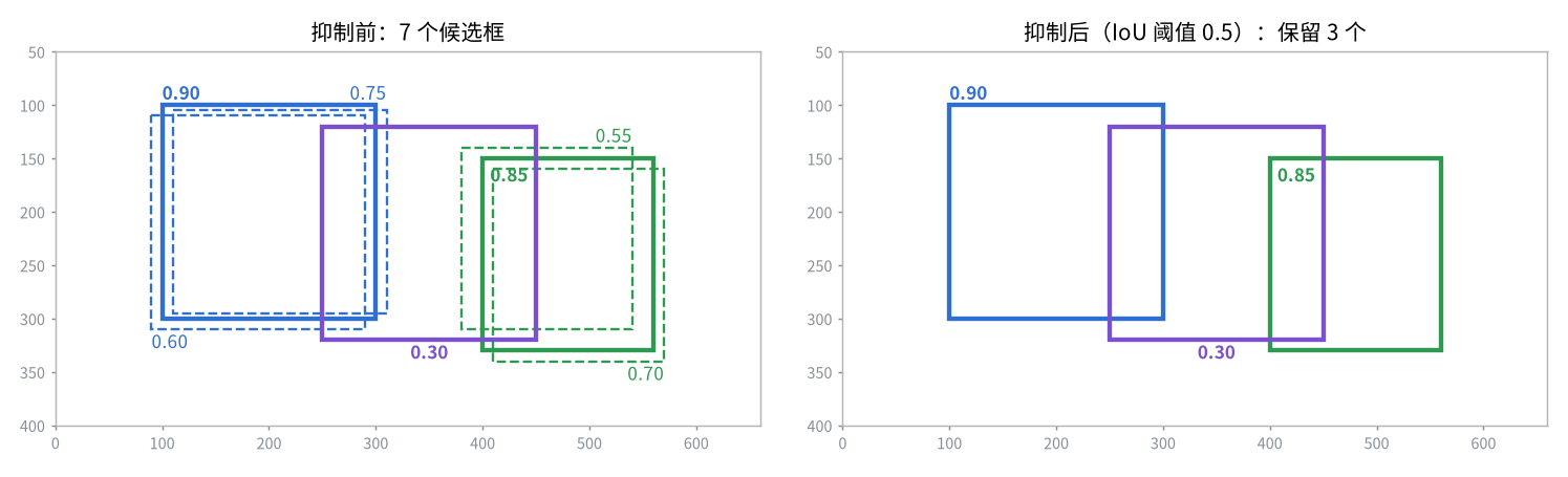
检测网络会在同一个目标附近输出多个位置相近的框。非极大值抑制(Non-Maximum Suppression,NMS)只保留其中分数最高的一个:
- 把所有框按分数从高到低排列
- 取出分数最高的框,保留
- 删除剩余的框中与它的 IoU 超过阈值的框
- 对剩下的框重复第 2、3 步,直到没有框为止
1
2
3
4
5
6
7
8
9
10
11
12
13
14
15
16
17
18
19
20
21
22
23
24
25
26
27
28
29
30
31
32
33
34
35
import torch
from torchvision.ops import box_iou, nms


def simple_nms(boxes, scores, iou_threshold):
    order = scores.argsort(descending=True)  # 按分数从高到低排列
    keep = []
    while order.numel() > 0:
        best = order[0]
        keep.append(best.item())
        if order.numel() == 1:
            break
        # 与当前分数最高的框重叠超过阈值的框被抑制
        overlap = box_iou(boxes[best][None], boxes[order[1:]])[0]
        order = order[1:][overlap <= iou_threshold]
    return torch.tensor(keep)


boxes = torch.tensor([
    [100., 100., 300., 300.],  # 目标 1 附近的三个框
    [110., 105., 310., 295.],
    [ 90., 110., 290., 310.],
    [400., 150., 560., 330.],  # 目标 2 附近的三个框
    [410., 160., 570., 340.],
    [380., 140., 540., 310.],
    [250., 120., 450., 320.],  # 夹在两个目标之间的框
])
scores = torch.tensor([0.90, 0.75, 0.60, 0.85, 0.70, 0.55, 0.30])

print(simple_nms(boxes, scores, iou_threshold=0.5))  # tensor([0, 3, 6])
print(nms(boxes, scores, iou_threshold=0.5))         # tensor([0, 3, 6])

# 不同阈值下保留的框
for threshold in [0.1, 0.3, 0.5, 0.7, 0.9]:
    print(threshold, nms(boxes, scores, threshold).tolist())
nms返回的是保留下来的框的下标,按分数从高到低排列,不是框本身
IoU 阈值的影响
上面的代码最后在不同阈值下运行了nms,7 个框中,0、1、2 属于第一个目标,3、4、5 属于第二个目标,6 夹在两个目标之间,与框 0 的 IoU 为 0.13
1
2
3
4
5
0.1 [0, 3]
0.3 [0, 3, 6]
0.5 [0, 3, 6]
0.7 [0, 3, 5, 6]
0.9 [0, 3, 1, 4, 2, 5, 6]
| 阈值 | 效果 |
|---|---|
| 过低 | 相邻或互相遮挡的不同目标被当作重复框删除,如 0.1 时的框 6 |
| 过高 | 同一个目标保留多个框,如 0.7 时的框 5、0.9 时的全部 |
常用的取值在 0.45 到 0.7 之间。目标密集、互相遮挡多的场景(人群、货架)适当调高,目标稀疏的场景可以调低
多个类别
nms不区分类别。两个类别不同的目标重叠在一起时(骑自行车的人和自行车),分数低的会被误删。batched_nms多接收一个类别编号,只在同一类别内部做抑制
1
2
3
4
5
6
7
8
9
10
11
12
13
14
15
16
17
18
import torch
from torchvision.ops import batched_nms, nms

# 两个几乎重合的框,类别不同(例如人和他骑的自行车)
boxes = torch.tensor([
    [100., 100., 300., 300.],
    [105., 105., 305., 305.],
    [102.,  98., 298., 302.],
])
scores = torch.tensor([0.90, 0.80, 0.70])
labels = torch.tensor([0, 1, 0])

print(nms(boxes, scores, iou_threshold=0.5))                  # tensor([0]),不同类别的框被误删
print(batched_nms(boxes, scores, labels, iou_threshold=0.5))  # tensor([0, 1])

# batched_nms 的做法:给每个类别的框加上一个足够大的偏移,使不同类别的框互不重叠
offset = labels[:, None] * (boxes.max() + 1)
print(nms(boxes + offset, scores, iou_threshold=0.5))         # tensor([0, 1])
锚框与无锚框
特征图上的格子
检测网络的骨干部分把图像逐步下采样,输入图像的边长与特征图的边长之比称为步幅。特征图上的一个格子对应输入图像上边长为步幅的一块区域,检测头在每个格子上各做一次预测。特征图大小的计算见PyTorch CNN
多数检测器同时使用几层不同步幅的特征图:步幅小的特征图格子密,负责小目标;步幅大的特征图感受野大,负责大目标。以 320x320 的输入为例
| 步幅 | 特征图大小 | 格子数 | 负责的目标 |
|---|---|---|---|
| 8 | 40x40 | 1600 | 小 |
| 16 | 20x20 | 400 | 中 |
| 32 | 10x10 | 100 | 大 |
锚框
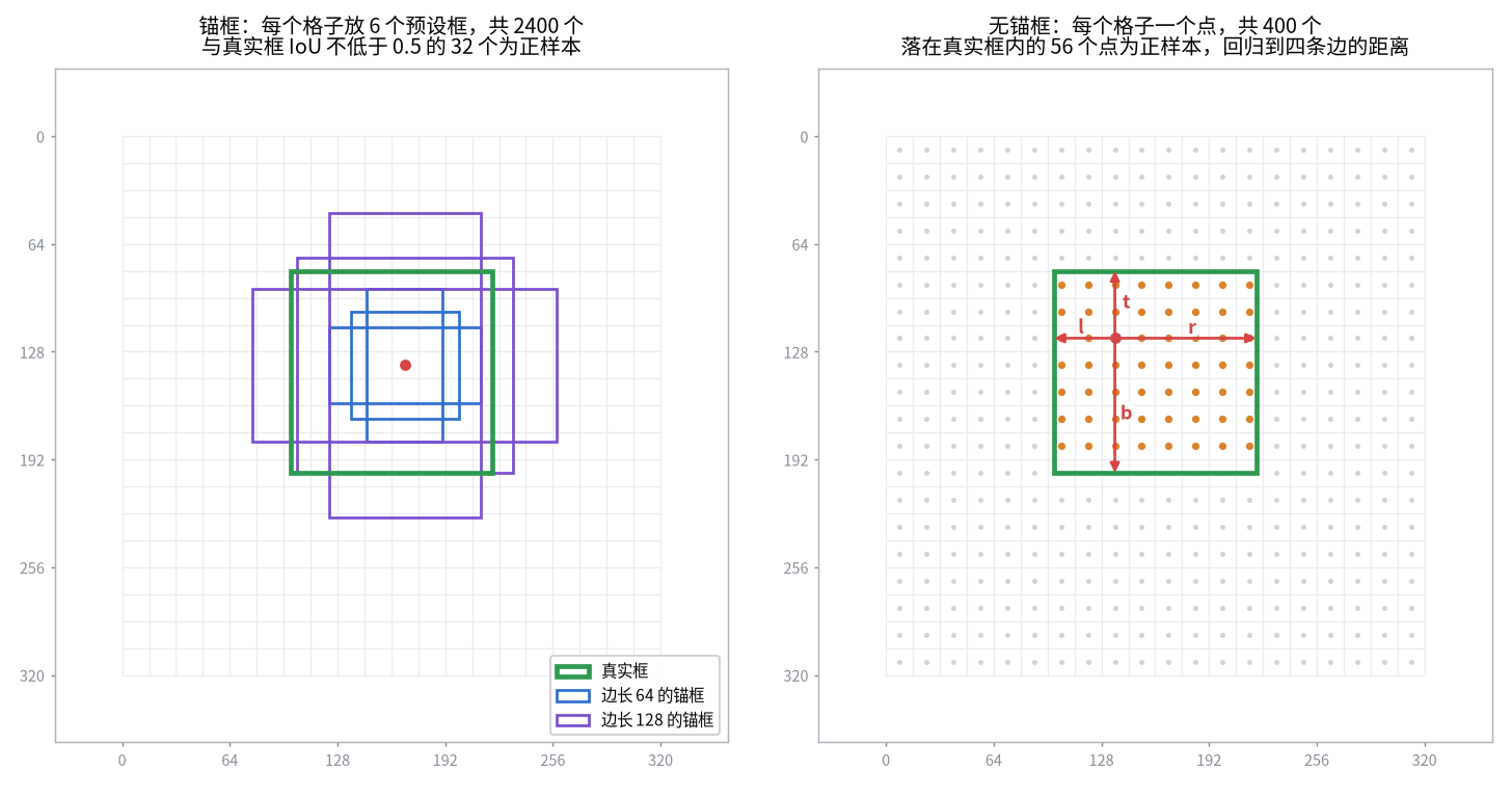
锚框(anchor)是在每个格子中心预先放置的一组大小和宽高比固定的框。网络不直接预测边界框,而是预测每个锚框相对于真实框的偏移量,以及这个锚框属于各个类别的分数
1
2
3
4
5
6
7
8
9
10
11
12
13
14
15
16
17
18
19
20
21
22
23
24
25
26
27
28
29
30
31
32
import torch
from torchvision.ops import box_iou


def make_anchors(feature_size, stride, sizes, ratios):
    """在特征图的每个格子中心放置 len(sizes) * len(ratios) 个锚框,返回 (H * W * A, 4),xyxy 格式"""
    height, width = feature_size
    # 每个格子的中心在输入图像上的坐标
    cy = (torch.arange(height) + 0.5) * stride
    cx = (torch.arange(width) + 0.5) * stride
    cy, cx = torch.meshgrid(cy, cx, indexing='ij')
    centers = torch.stack([cx, cy], dim=-1).reshape(-1, 1, 2)  # (H * W, 1, 2)

    # 面积保持为 size 的平方,宽高比为 ratio(高 / 宽)
    sizes = torch.tensor(sizes, dtype=torch.float32)
    ratios = torch.tensor(ratios, dtype=torch.float32)
    w = (sizes[:, None] / ratios.sqrt()[None, :]).reshape(-1)
    h = (sizes[:, None] * ratios.sqrt()[None, :]).reshape(-1)
    half = torch.stack([w, h], dim=-1)[None] / 2               # (1, A, 2)

    return torch.cat([centers - half, centers + half], dim=-1).reshape(-1, 4)


# 320x320 的输入,步幅 16 的特征图大小为 20x20
anchors = make_anchors((20, 20), stride=16, sizes=[64, 128], ratios=[0.5, 1.0, 2.0])
print(anchors.shape)  # torch.Size([2400, 4])
print(anchors[:3])    # 第一个格子上边长为 64 的 3 个锚框

# 与真实框的 IoU 不低于 0.5 的锚框作为正样本
gt = torch.tensor([[100., 80., 220., 200.]])
overlap = box_iou(anchors, gt)[:, 0]
print((overlap >= 0.5).sum().item(), '/', len(anchors))  # 32 / 2400
1
2
3
4
5
torch.Size([2400, 4])
tensor([[-37.2548, -14.6274,  53.2548,  30.6274],
        [-24.0000, -24.0000,  40.0000,  40.0000],
        [-14.6274, -37.2548,  30.6274,  53.2548]])
32 / 2400
靠近图像边缘的锚框会超出图像,坐标为负是正常的。训练时用 IoU 把锚框分配给真实框,2400 个锚框中只有 32 个是正样本,其余都是背景,这种正负样本的极度不平衡正是后面焦点损失要解决的问题
无锚框
无锚框(anchor-free)的检测器不预设框,每个格子只对应一个点,直接预测这个点到边界框四条边的距离,或者预测中心点的位置和宽高
1
2
3
4
5
6
7
8
9
10
11
12
13
14
15
16
17
18
19
20
21
22
23
24
import torch


def make_points(feature_size, stride):
    """特征图每个格子的中心在输入图像上的坐标,返回 (H * W, 2)"""
    height, width = feature_size
    cy = (torch.arange(height) + 0.5) * stride
    cx = (torch.arange(width) + 0.5) * stride
    cy, cx = torch.meshgrid(cy, cx, indexing='ij')
    return torch.stack([cx, cy], dim=-1).reshape(-1, 2)


points = make_points((20, 20), stride=16)
print(points.shape)  # torch.Size([400, 2])
print(points[:3].tolist())  # [[8.0, 8.0], [24.0, 8.0], [40.0, 8.0]]

# 落在真实框内部的点作为正样本,回归目标是该点到框四条边的距离
gt = torch.tensor([100., 80., 220., 200.])
left, top = points[:, 0] - gt[0], points[:, 1] - gt[1]
right, bottom = gt[2] - points[:, 0], gt[3] - points[:, 1]
distances = torch.stack([left, top, right, bottom], dim=-1)  # (H * W, 4)
inside = distances.min(dim=-1).values > 0
print(inside.sum().item(), '/', len(points))    # 56 / 400
print(points[inside][0], distances[inside][0])  # tensor([104.,  88.]) tensor([  4.,   8., 116., 112.])
| 对比项 | 锚框 | 无锚框 |
|---|---|---|
| 每个格子的预测 | 多个,每个锚框一组 | 一个 |
| 回归的内容 | 相对于锚框的偏移和缩放 | 到四条边的距离,或中心点和宽高 |
| 正样本的确定 | 锚框与真实框的 IoU | 点是否落在真实框内或中心附近 |
| 需要设定 | 锚框的大小和宽高比,与数据集有关 | 不需要 |
| 代表模型 | Faster R-CNN、SSD、RetinaNet、YOLOv3 至 v5 | FCOS、CenterNet、YOLOX、YOLOv8 及之后 |
锚框的大小需要与数据集中目标的大小相符,否则没有锚框能与真实框达到足够的 IoU,这些目标就学不到。换数据集时需要重新统计,YOLOv5 的做法是对标注框的宽高做聚类。无锚框的方式省去了这一步,也减少了输出的数量,较新的检测器大多采用
检测头的输出与解码
输出的形状
单阶段检测器的检测头通常就是若干个卷积层,输出仍然是一张特征图,每个格子的通道中依次存放边界框和类别的预测值。把它变成边界框的过程称为解码
| 类型 | 每个格子的通道数 | 含义 |
|---|---|---|
| 无锚框 | 4 + C | 4 个边界框参数,C 个类别分数 |
| 锚框,A 个 | A x (4 + C) | 每个锚框各一组 |
| 带目标置信度的锚框 | A x (5 + C) | 多一个表示是否有目标的分数,如 YOLOv5 |
下面以无锚框、三层特征图的检测头为例,用随机张量代替骨干网络的输出,完成从原始输出到最终结果的全过程
1
2
3
4
5
6
7
8
9
10
11
12
13
14
15
16
17
18
19
20
21
22
23
24
25
26
27
28
29
30
31
32
33
34
35
36
37
38
39
40
41
42
43
44
45
46
47
48
49
50
51
52
53
54
55
56
57
58
59
60
61
62
63
64
65
import torch
from torch import nn
from torchvision.ops import batched_nms

torch.manual_seed(0)
num_classes = 3
strides = [8, 16, 32]

# 320x320 的输入经过骨干网络后得到的三层特征图,这里用随机张量代替
features = [torch.randn(2, 64, 320 // s, 320 // s) for s in strides]

# 检测头:每个位置输出 4 个距离和 num_classes 个类别分数
head = nn.Conv2d(64, 4 + num_classes, kernel_size=1)
outputs = [head(f) for f in features]
for out in outputs:
    print(out.shape)
# torch.Size([2, 7, 40, 40])
# torch.Size([2, 7, 20, 20])
# torch.Size([2, 7, 10, 10])


def decode(outputs, strides):
    boxes, logits = [], []
    for out, stride in zip(outputs, strides):
        n, c, h, w = out.shape
        out = out.permute(0, 2, 3, 1).reshape(n, h * w, c)  # (N, H * W, 4 + C)

        cy = (torch.arange(h) + 0.5) * stride
        cx = (torch.arange(w) + 0.5) * stride
        cy, cx = torch.meshgrid(cy, cx, indexing='ij')
        points = torch.stack([cx, cy], dim=-1).reshape(-1, 2)  # (H * W, 2)

        # 前 4 个通道是到左、上、右、下四条边的距离,以步幅为单位,取指数保证为正
        distances = out[..., :4].exp() * stride
        x1y1 = points - distances[..., :2]
        x2y2 = points + distances[..., 2:]
        boxes.append(torch.cat([x1y1, x2y2], dim=-1))
        logits.append(out[..., 4:])
    return torch.cat(boxes, dim=1), torch.cat(logits, dim=1)


boxes, logits = decode(outputs, strides)
print(boxes.shape, logits.shape)  # torch.Size([2, 2100, 4]) torch.Size([2, 2100, 3])


def postprocess(boxes, logits, score_threshold=0.5, iou_threshold=0.5, image_size=(320, 320)):
    """处理一张图像:boxes 为 (M, 4),logits 为 (M, C)"""
    scores, labels = logits.sigmoid().max(dim=-1)  # 每个位置取分数最高的类别
    keep = scores > score_threshold
    boxes, scores, labels = boxes[keep], scores[keep], labels[keep]

    # 把超出图像的部分裁掉
    boxes[:, 0::2] = boxes[:, 0::2].clamp(0, image_size[1])
    boxes[:, 1::2] = boxes[:, 1::2].clamp(0, image_size[0])

    keep = batched_nms(boxes, scores, labels, iou_threshold)
    return boxes[keep], scores[keep], labels[keep]


with torch.no_grad():
    for i in range(2):  # 每张图像保留的框数不同,只能逐张处理
        b, s, l = postprocess(boxes[i], logits[i])
        print(b.shape, s.shape, l.shape)
# torch.Size([1626, 4]) torch.Size([1626]) torch.Size([1626])
# torch.Size([1618, 4]) torch.Size([1618]) torch.Size([1618])
解码分为三步:
- 把每一层的输出从 (N, 4 + C, H, W) 变为 (N, H x W, 4 + C),每一行是一个格子的预测
- 生成每个格子的中心点坐标,与预测的距离组合成
xyxy格式的框,乘以步幅还原到输入图像的尺度 - 把各层的结果拼接在一起。320x320 的输入共有 1600 + 400 + 100 = 2100 个预测
之后的后处理是所有检测器通用的:类别分数经过 sigmoid,按分数阈值过滤,再做非极大值抑制。这里的权重是随机的,分数没有意义,所以剩下的框很多;训练好的模型绝大多数位置的分数接近 0,过滤后只剩几个到几十个
permute不能省略。直接对 (N, 4 + C, H, W) 做reshape会把通道和空间位置混在一起,形状正确但内容是错的- 生成网格时
torch.meshgrid要写indexing='ij',返回的顺序是先$y$后$x$,而框的坐标是先$x$后$y$,两者容易弄反。长宽不相等的输入最容易暴露这个问题 - 每张图像保留下来的框数量不同,后处理只能逐张图像进行,结果是列表而不是一个张量
不同模型的解码公式不同(锚框的偏移、距离的分布等),导出为 ONNX 的模型有些已经包含解码,有些没有,使用前要看清输出的形状。例如 YOLOv8 导出后的输出为 (N, 4 + C, 8400),其中 8400 是 640x640 的输入在步幅 8、16、32 下的格子总数 6400 + 1600 + 400,边界框已经解码为cxcywh,但没有做非极大值抑制
损失函数
检测的损失由两部分相加:分类损失针对所有位置,边界框回归损失只针对正样本
分类:焦点损失
单阶段检测器的每个位置都要分类,其中绝大多数是容易区分的背景。每个背景的损失虽然小,但数量太多,加起来会淹没少数正样本的损失。焦点损失(Focal Loss)在交叉熵前乘以一个系数,把已经分对的样本的损失压低
\[FL(p_t) = -\alpha_t (1 - p_t)^{\gamma} \log(p_t)\]其中$p_t$是模型对正确答案给出的概率,分得越对越接近 1,系数越接近 0
| 参数 | 含义 | 常用值 |
|---|---|---|
gamma | 压低容易样本的力度,0 时退化为交叉熵 | 2 |
alpha | 正样本的权重,负样本的权重为1 - alpha,设为 -1 表示不使用 | 0.25 |
1
2
3
4
5
6
7
8
9
10
11
12
13
14
15
16
17
18
19
20
21
22
23
24
25
26
27
28
29
import torch
import torch.nn.functional as F
from torchvision.ops import sigmoid_focal_loss

torch.set_printoptions(precision=4, sci_mode=False)

# 一个正样本和四个负样本,后面的负样本预测得越来越差
probability = torch.tensor([0.9, 0.1, 0.3, 0.5, 0.9])
target = torch.tensor([1.0, 0.0, 0.0, 0.0, 0.0])
logits = torch.logit(probability)  # 损失函数接收的是 sigmoid 之前的值

bce = F.binary_cross_entropy_with_logits(logits, target, reduction='none')
focal = sigmoid_focal_loss(logits, target, alpha=0.25, gamma=2.0, reduction='none')
print(bce)    # tensor([0.1054, 0.1054, 0.3567, 0.6931, 2.3026])
print(focal)  # tensor([0.0003, 0.0008, 0.0241, 0.1300, 1.3988])

# 手动计算
p_t = torch.where(target == 1, probability, 1 - probability)  # 预测正确的概率
alpha_t = torch.where(target == 1, 0.25, 0.75)
print(alpha_t * (1 - p_t) ** 2 * bce)  # tensor([0.0003, 0.0008, 0.0241, 0.1300, 1.3988])

# 1 个没预测好的正样本和 2399 个容易的负样本
logits = torch.cat([torch.tensor([-1.0]), torch.full((2399,), -3.0)])
target = torch.zeros(2400)
target[0] = 1.0
bce = F.binary_cross_entropy_with_logits(logits, target, reduction='none')
focal = sigmoid_focal_loss(logits, target, alpha=0.25, gamma=2.0, reduction='none')
print(f'BCE    正样本 {bce[0]:.4f}  负样本合计 {bce[1:].sum():.4f}')
print(f'Focal  正样本 {focal[0]:.4f}  负样本合计 {focal[1:].sum():.4f}')
1
2
3
4
5
tensor([0.1054, 0.1054, 0.3567, 0.6931, 2.3026])
tensor([0.0003, 0.0008, 0.0241, 0.1300, 1.3988])
tensor([0.0003, 0.0008, 0.0241, 0.1300, 1.3988])
BCE    正样本 1.3133  负样本合计 116.5610
Focal  正样本 0.1755  负样本合计 0.1966
预测概率为 0.1 的容易负样本,损失从 0.1054 降到 0.0008,缩小了一百多倍;预测错的负样本(概率 0.9)只从 2.3026 降到 1.3988。在 1 个正样本对 2399 个负样本的例子中,交叉熵下负样本的损失之和是正样本的近 90 倍,焦点损失下两者相当
sigmoid_focal_loss接收的是 sigmoid 之前的值,不要先做 sigmoidtargets是与输入形状相同的浮点张量(每个类别一个 0 或 1),不是类别编号reduction默认为'none',返回每个元素的损失。通常求和后除以正样本的个数,而不是取平均,否则损失会被大量负样本稀释
边界框回归
| 损失 | 计算方式 | 特点 |
|---|---|---|
| L1 | 坐标差的绝对值 | 与框的大小有关,大目标的损失大 |
| Smooth L1 | 差值小时为平方,差值大时为绝对值 | 对异常值不敏感,Faster R-CNN、SSD 使用 |
| IoU 类(GIoU、DIoU、CIoU) | 1 减去对应的 IoU | 与框的大小无关,直接优化评价指标 |
1
2
3
4
5
6
7
8
9
10
11
12
13
14
15
16
17
18
19
20
21
22
23
import torch
import torch.nn.functional as F
from torchvision.ops import box_iou, complete_box_iou_loss, distance_box_iou_loss, generalized_box_iou_loss

# 一大一小两个目标,预测框都向右下偏移了边长的 10%
target = torch.tensor([[100., 100., 300., 300.], [100., 100., 120., 120.]])
pred = torch.tensor([[120., 120., 320., 320.], [102., 102., 122., 122.]])

print(F.l1_loss(pred, target, reduction='none').sum(dim=1))         # tensor([80.,  8.])
print(F.smooth_l1_loss(pred, target, reduction='none').sum(dim=1))  # tensor([78.,  6.])
print(generalized_box_iou_loss(pred, target))                       # tensor([0.3359, 0.3359])
print(distance_box_iou_loss(pred, target))                          # tensor([0.3276, 0.3276])
print(complete_box_iou_loss(pred, target))                          # tensor([0.3276, 0.3276])

# 预测框与真实框不相交时,1 - IoU 的梯度为 0,GIoU 损失仍然有梯度
target = torch.tensor([[100., 100., 300., 300.]])
pred = torch.tensor([[320., 120., 420., 280.]], requires_grad=True)

iou_loss = 1 - box_iou(pred, target)[0, 0]
print(iou_loss.item(), torch.autograd.grad(iou_loss, pred)[0])

giou_loss = generalized_box_iou_loss(pred, target, reduction='sum')
print(giou_loss.item(), torch.autograd.grad(giou_loss, pred)[0])
1
2
3
4
5
6
7
tensor([80.,  8.])
tensor([78.,  6.])
tensor([0.3359, 0.3359])
tensor([0.3276, 0.3276])
tensor([0.3276, 0.3276])
1.0 tensor([[0., 0., 0., 0.]])
1.125 tensor([[ 0.0025,  0.0016,  0.0002, -0.0016]])
两个预测框偏移的比例相同,L1 损失相差 10 倍,IoU 类的损失则完全相同。使用 L1 类损失的检测器通常不直接回归坐标,而是回归相对于锚框大小归一化后的偏移量,以消除尺度的影响
预测框与真实框不相交时,1 - IoU 的梯度全为 0,网络得不到任何更新方向;GIoU 损失仍然有梯度,其中左边界的梯度为正,梯度下降会让左边界向左移动,靠近真实框
generalized_box_iou_loss等三个函数接收的是一一对应的两组框,形状都是 (N, 4),返回 (N,);generalized_box_iou等函数则返回 (N, M) 的矩阵。两组函数名字相近,用途不同
评价指标 mAP
TP、FP 与 FN
分类任务中精确率和召回率的含义见Evaluation Metrics。检测任务没有现成的对错,需要先用 IoU 把预测框与真实框配对
| 名称 | 含义 |
|---|---|
| TP | 预测框与一个尚未被匹配的同类别真实框的 IoU 不低于阈值 |
| FP | 预测框没有匹配到真实框,或者匹配的真实框已经被分数更高的框占用 |
| FN | 没有被任何预测框匹配到的真实框 |
精确率是 TP 占所有预测框的比例,召回率是 TP 占所有真实框的比例。检测任务中没有 TN,因为不存在可以计数的背景框
AP 的计算
精确率和召回率都依赖分数阈值:阈值高,留下的框少而准;阈值低,找到的目标多但误检也多。AP(Average Precision)把所有阈值都考虑进来:
- 把一个类别在所有图像上的预测框放在一起,按分数从高到低排列
- 从前往后逐个加入预测框,每加入一个就计算一次精确率和召回率,得到精确率-召回率曲线
- 把曲线上每个点的精确率替换为它右侧的最大值,得到单调下降的包络
- AP 是包络下的面积
1
2
3
4
5
6
7
8
9
10
11
12
13
14
15
16
17
18
19
20
21
22
23
24
25
26
27
28
29
30
31
32
33
34
35
36
37
38
39
40
41
42
43
44
45
46
47
48
49
50
51
52
53
54
55
56
57
58
59
60
61
62
63
64
65
66
67
68
69
70
71
72
import torch
from torchvision.ops import box_iou

# 3 张图像、1 个类别、共 5 个真实框
targets = [
    torch.tensor([[50., 50., 150., 150.], [200., 80., 300., 200.]]),
    torch.tensor([[30., 40., 130., 160.], [180., 60., 280., 180.]]),
    torch.tensor([[100., 100., 220., 220.]]),
]
# 每张图像的预测框和分数
predictions = [
    (torch.tensor([[52., 48., 152., 148.], [210., 100., 310., 215.], [400., 300., 460., 380.]]),
     torch.tensor([0.95, 0.60, 0.80])),
    (torch.tensor([[35., 45., 128., 150.], [60., 70., 160., 190.], [185., 70., 290., 185.]]),
     torch.tensor([0.90, 0.70, 0.50])),
    (torch.tensor([[120., 125., 240., 245.], [300., 50., 360., 110.]]),
     torch.tensor([0.85, 0.40])),
]


def match(predictions, targets, iou_threshold):
    """判断每个预测框是 TP 还是 FP,返回所有图像的分数和 TP 标记"""
    all_scores, all_tp = [], []
    for (boxes, scores), gt in zip(predictions, targets):
        overlap = box_iou(boxes, gt)  # (预测框个数, 真实框个数)
        used = torch.zeros(len(gt), dtype=torch.bool)
        tp = torch.zeros(len(boxes), dtype=torch.bool)
        for i in scores.argsort(descending=True):  # 分数高的预测框优先匹配
            candidate = overlap[i].clone()
            candidate[used] = 0                    # 每个真实框只能被匹配一次
            best = candidate.argmax()
            if candidate[best] >= iou_threshold:
                tp[i] = True
                used[best] = True
        all_scores.append(scores)
        all_tp.append(tp)
    return torch.cat(all_scores), torch.cat(all_tp)


def average_precision(scores, tp, num_targets):
    order = scores.argsort(descending=True)
    tp = tp[order].float()
    tp_count = tp.cumsum(0)
    fp_count = (1 - tp).cumsum(0)
    recall = tp_count / num_targets
    precision = tp_count / (tp_count + fp_count)

    # 包络:每个位置的精确率取它右侧的最大值,消除曲线的锯齿
    envelope = precision.flip(0).cummax(0).values.flip(0)
    # 包络下的面积
    previous = torch.cat([torch.zeros(1), recall[:-1]])
    ap = ((recall - previous) * envelope).sum()
    return ap.item(), recall, precision, envelope


num_targets = sum(len(gt) for gt in targets)
scores, tp = match(predictions, targets, iou_threshold=0.5)
ap, recall, precision, envelope = average_precision(scores, tp, num_targets)

order = scores.argsort(descending=True)
print('分数  ', [round(v, 2) for v in scores[order].tolist()])
print('TP    ', tp[order].int().tolist())
print('精确率', [round(v, 2) for v in precision.tolist()])
print('召回率', [round(v, 2) for v in recall.tolist()])
print(f'AP50 = {ap:.4f}')

# 在多个 IoU 阈值下分别计算再取平均
thresholds = [0.5 + 0.05 * i for i in range(10)]
aps = [average_precision(*match(predictions, targets, t), num_targets)[0] for t in thresholds]
print('各阈值的 AP', [round(v, 3) for v in aps])
print(f'AP75 = {aps[5]:.4f}')
print(f'AP@[0.5:0.95] = {sum(aps) / len(aps):.4f}')
1
2
3
4
5
6
7
8
分数   [0.95, 0.9, 0.85, 0.8, 0.7, 0.6, 0.5, 0.4]
TP     [1, 1, 0, 0, 0, 1, 1, 0]
精确率 [1.0, 1.0, 0.67, 0.5, 0.4, 0.5, 0.57, 0.5]
召回率 [0.2, 0.4, 0.4, 0.4, 0.4, 0.6, 0.8, 0.8]
AP50 = 0.6286
各阈值的 AP [0.629, 0.629, 0.629, 0.486, 0.486, 0.486, 0.4, 0.2, 0.2, 0.0]
AP75 = 0.4857
AP@[0.5:0.95] = 0.4143
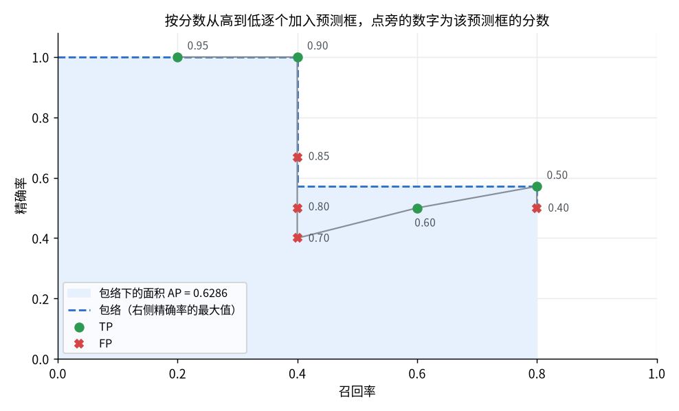
- 分数 0.85 的预测框与真实框的 IoU 为 0.49,看上去框住了目标,在 0.5 的阈值下仍然是 FP
- 分数 0.70 的预测框与一个真实框的 IoU 只有 0.36,而且该真实框已经被分数 0.90 的框匹配,是 FP。没有做好非极大值抑制时,重复的框都会像这样被计为 FP
- 5 个真实框中有 1 个始终没有被检测到,召回率最高只到 0.8,曲线在 0.8 之后的面积为 0
- 排在前面的 FP 比排在后面的 FP 对 AP 的影响大得多,所以分数的排序质量与框的位置同样重要
常用的指标
| 指标 | 含义 |
|---|---|
| AP50 | IoU 阈值为 0.5 时的 AP,Pascal VOC 使用 |
| AP75 | IoU 阈值为 0.75 时的 AP,对定位精度要求更高 |
| AP@[0.5:0.95] | 阈值从 0.5 到 0.95 每隔 0.05 取一个,10 个 AP 的平均,COCO 的主要指标 |
| mAP | 对每个类别分别计算 AP,再对所有类别取平均 |
| AP small / medium / large | 按目标面积分组统计,分界为 32x32 和 96x96 像素 |
COCO 中通常把 mAP 直接写作 AP,指的是对类别和 10 个 IoU 阈值都取平均后的结果
使用 torchmetrics
torchmetrics.detection.MeanAveragePrecision实现了 COCO 的评价方式,需要另外安装pycocotools。下面用它计算与手动计算时相同的数据
1
2
3
4
5
6
7
8
9
10
11
12
13
14
15
16
17
18
19
20
21
22
23
24
25
26
27
import torch
from torchmetrics.detection import MeanAveragePrecision

# 与上面手动计算时相同的数据
targets = [
    torch.tensor([[50., 50., 150., 150.], [200., 80., 300., 200.]]),
    torch.tensor([[30., 40., 130., 160.], [180., 60., 280., 180.]]),
    torch.tensor([[100., 100., 220., 220.]]),
]
predictions = [
    (torch.tensor([[52., 48., 152., 148.], [210., 100., 310., 215.], [400., 300., 460., 380.]]),
     torch.tensor([0.95, 0.60, 0.80])),
    (torch.tensor([[35., 45., 128., 150.], [60., 70., 160., 190.], [185., 70., 290., 185.]]),
     torch.tensor([0.90, 0.70, 0.50])),
    (torch.tensor([[120., 125., 240., 245.], [300., 50., 360., 110.]]),
     torch.tensor([0.85, 0.40])),
]

# 预测和标注都是字典的列表,每张图像一个字典,这里只有一个类别,编号为 0
preds = [{ 'boxes': boxes, 'scores': scores, 'labels': torch.zeros(len(boxes), dtype=torch.long) } for boxes, scores in predictions]
target = [{ 'boxes': boxes, 'labels': torch.zeros(len(boxes), dtype=torch.long) } for boxes in targets]

metric = MeanAveragePrecision(box_format='xyxy')
metric.update(preds, target)
result = metric.compute()
for key in ['map_50', 'map_75', 'map', 'mar_100']:
    print(f'{key:8s}{result[key].item():.4f}')
1
2
3
4
map_50  0.6266
map_75  0.4866
map     0.4161
mar_100 0.5000
| 指标 | 手动计算 | torchmetrics |
|---|---|---|
| AP50 | 0.6286 | 0.6266 |
| AP75 | 0.4857 | 0.4866 |
| AP@[0.5:0.95] | 0.4143 | 0.4161 |
两者在小数点后第三位有差别,原因是面积的算法不同:COCO 的官方实现不直接计算包络下的面积,而是在 0 到 1 之间取 101 个等间隔的召回率,对包络采样后取平均。比较不同模型时要使用同一套评价代码
mar_100是每张图像最多取 100 个预测框时的平均召回率,同样对 10 个 IoU 阈值取平均。这个例子中各阈值下的召回率依次为 0.8、0.8、0.8、0.6、0.6、0.6、0.4、0.2、0.2、0,平均为 0.5
使用预训练检测器
推理
torchvision.models.detection提供了在 COCO 上预训练的检测模型,后处理已经包含在模型内部,输出直接是最终的检测结果
| 模型 | 类型 | 特点 |
|---|---|---|
fasterrcnn_resnet50_fpn_v2 | 两阶段,锚框 | 精度高,速度慢 |
fasterrcnn_mobilenet_v3_large_320_fpn | 两阶段,锚框 | 轻量,适合 CPU |
retinanet_resnet50_fpn_v2 | 单阶段,锚框 | 使用焦点损失 |
fcos_resnet50_fpn | 单阶段,无锚框 | 回归到四条边的距离 |
ssdlite320_mobilenet_v3_large | 单阶段,锚框 | 最轻量 |
为了让结果可以重复,下面用代码画一张合成的街景作为测试图像,左边是红绿灯,右边是停车标志
1
2
3
4
5
6
7
8
9
10
11
12
13
14
15
16
17
18
19
20
21
22
23
24
25
26
27
28
29
import math

from PIL import Image, ImageDraw


def make_scene(width=512, height=600):
    """画一张合成的街景:左边是红绿灯,右边是停车标志"""
    image = Image.new('RGB', (width, height), (150, 190, 225))  # 天空
    draw = ImageDraw.Draw(image)
    draw.rectangle([0, 430, width, height], fill=(120, 125, 130))  # 路面

    # 红绿灯:灯杆、灯箱和三盏灯,只有红灯亮
    draw.rectangle([100, 330, 120, 490], fill=(60, 60, 60))
    draw.rounded_rectangle([60, 60, 160, 330], radius=20, fill=(35, 35, 35))
    for center_y, color in zip([105, 195, 285], [(230, 40, 40), (90, 80, 20), (20, 80, 30)]):
        draw.ellipse([78, center_y - 32, 142, center_y + 32], fill=color)

    # 停车标志:立柱、白边和红色的八边形
    def octagon(radius):
        return [(340 + radius * math.cos(math.radians(22.5 + 45 * k)), 230 + radius * math.sin(math.radians(22.5 + 45 * k))) for k in range(8)]

    draw.rectangle([334, 230, 346, 520], fill=(170, 170, 170))
    draw.polygon(octagon(140), fill=(255, 255, 255))
    draw.polygon(octagon(129), fill=(200, 25, 30))
    return image


if __name__ == '__main__':
    make_scene().save('scene.png')
1
2
3
4
5
6
7
8
9
10
11
12
13
14
15
16
17
18
19
20
21
22
23
24
25
import torch
from torchvision.models.detection import FasterRCNN_MobileNet_V3_Large_320_FPN_Weights, fasterrcnn_mobilenet_v3_large_320_fpn
from torchvision.transforms.functional import pil_to_tensor

from scene import make_scene

weights = FasterRCNN_MobileNet_V3_Large_320_FPN_Weights.DEFAULT
model = fasterrcnn_mobilenet_v3_large_320_fpn(weights=weights)
model.eval()

image = make_scene()  # 合成的街景,宽 512、高 600
x = pil_to_tensor(image).float() / 255  # (3, H, W),取值范围 [0, 1]
print(x.shape)  # torch.Size([3, 600, 512])

with torch.no_grad():
    outputs = model([x])  # 输入是图像的列表,每张图像的大小可以不同

output = outputs[0]       # 每张图像对应一个字典
for key, value in output.items():
    print(key, value.shape, value.dtype)

categories = weights.meta['categories']
keep = output['scores'] > 0.5
for box, label, score in zip(output['boxes'][keep], output['labels'][keep], output['scores'][keep]):
    print(f'{categories[label]:15s}{score:.3f}  {[round(v) for v in box.tolist()]}')
1
2
3
4
5
6
torch.Size([3, 600, 512])
boxes torch.Size([2, 4]) torch.float32
labels torch.Size([2]) torch.int64
scores torch.Size([2]) torch.float32
stop sign      0.997  [215, 96, 471, 359]
traffic light  0.965  [54, 52, 165, 342]
| 键 | 形状 | 含义 |
|---|---|---|
boxes | (K, 4) | xyxy格式的绝对坐标,属于输入图像的坐标系 |
labels | (K,) | 类别编号,用weights.meta['categories']查名称 |
scores | (K,) | 置信度分数,已经从高到低排列 |
模型默认返回分数高于 0.05 的所有结果。这张合成图像很干净,只返回了 2 个框;真实图像上会有很多低分的误检,使用前需要按分数再过滤一次。阈值根据应用决定:漏检代价高时调低,误检代价高时调高
输入的要求
| 输入 | 结果 |
|---|---|
| 取值在 0 到 1 之间的浮点张量 | 正确,检测到 stop sign 和 traffic light |
| 取值在 0 到 255 之间的浮点张量 | 不报错,没有返回任何检测结果 |
| 自己先做了 ImageNet 的标准化 | 不报错,stop sign 的分数降到 0.979,traffic light 降到 0.276,按 0.5 过滤后漏检 |
uint8张量 | 抛出TypeError |
模型内部已经包含标准化和缩放,输入只需要除以 255。 重复做标准化或者忘记除以 255 都不会报错,只是结果不对,这是使用这些模型时最常见的错误
- 输入是三维张量的列表而不是一个四维张量,列表中的图像大小可以不同,模型内部会缩放并填充成一个批次
- 类别表共 91 项,编号 0 是
__background__,中间有若干N/A占位,实际只有 80 个类别。在自己的数据集上微调时,类别编号同样要从 1 开始,0 留给背景 - 必须调用
model.eval()。训练模式下模型的调用方式是model(images, targets),返回的是各项损失的字典而不是检测结果 - 训练时
targets中的边界框为xyxy格式的绝对坐标,宽或高为 0 的框会直接抛出AssertionError,数据增强后要把这样的框去掉
创建模型时可以修改后处理的参数
| 参数 | 默认值 | 含义 |
|---|---|---|
box_score_thresh | 0.05 | 低于该分数的结果不返回 |
box_nms_thresh | 0.5 | 非极大值抑制的 IoU 阈值 |
box_detections_per_img | 100 | 每张图像最多返回的结果个数 |
坐标映射
缩放与填充
检测网络的输入大小是固定的,相机图像需要先缩放。torchvision的检测模型在内部完成缩放,并把结果映射回原图;而自己做预处理的模型(导出为 ONNX 的模型、YOLO 系列)输出的坐标属于缩放后的图像,需要自己映射回去
| 方式 | 做法 | 映射回原图 |
|---|---|---|
| 直接拉伸 | 宽和高分别缩放到目标大小 | $x$和$y$分别除以各自的缩放比例 |
| 等比例缩放加填充 | 按较小的比例缩放,不足的部分用灰色填充 | 先减去填充量,再除以同一个缩放比例 |
直接拉伸会改变目标的宽高比,1920x1080 的图像拉伸成正方形后,目标在水平方向被压扁近一半。等比例缩放加填充(letterbox)保持宽高比不变,是 YOLO 系列的默认做法
1
2
3
4
5
6
7
8
9
10
11
12
13
14
15
16
17
18
19
20
21
22
23
24
25
26
27
28
29
30
31
32
33
34
35
36
37
38
39
40
41
42
import torch
import torch.nn.functional as F


def letterbox(image, size, fill=0.5):
    """把 (3, H, W) 的图像等比例缩放后填充到 size x size,返回新图像、缩放比例和左上角的填充量"""
    height, width = image.shape[1:]
    scale = min(size / height, size / width)
    new_height, new_width = round(height * scale), round(width * scale)
    resized = F.interpolate(image[None], size=(new_height, new_width), mode='bilinear', align_corners=False)[0]

    pad_left = (size - new_width) // 2
    pad_top = (size - new_height) // 2
    padding = (pad_left, size - new_width - pad_left, pad_top, size - new_height - pad_top)  # 左、右、上、下
    return F.pad(resized, padding, value=fill), scale, (pad_left, pad_top)


def to_letterbox(boxes, scale, pad):
    """原图上的框 -> 网络输入上的框:先缩放再平移"""
    offset = torch.tensor([pad[0], pad[1], pad[0], pad[1]])
    return boxes * scale + offset


def to_original(boxes, scale, pad, original_size):
    """网络输入上的框 -> 原图上的框:先减去填充再除以缩放比例,最后裁剪到图像范围内"""
    offset = torch.tensor([pad[0], pad[1], pad[0], pad[1]])
    boxes = (boxes - offset) / scale
    height, width = original_size
    boxes[:, 0::2] = boxes[:, 0::2].clamp(0, width)
    boxes[:, 1::2] = boxes[:, 1::2].clamp(0, height)
    return boxes


if __name__ == '__main__':
    image = torch.rand(3, 1080, 1920)  # 1920x1080 的相机图像
    resized, scale, pad = letterbox(image, 640)
    print(resized.shape, scale, pad)  # torch.Size([3, 640, 640]) 0.3333333333333333 (0, 140)

    boxes = torch.tensor([[600., 300., 1200., 900.]])
    mapped = to_letterbox(boxes, scale, pad)
    print(mapped)                                         # tensor([[200., 240., 400., 440.]])
    print(to_original(mapped, scale, pad, (1080, 1920)))  # tensor([[ 600.,  300., 1200.,  900.]])
映射回原图时的顺序与预处理相反:预处理是先缩放再平移,还原时先减去填充量再除以缩放比例。顺序弄反或者忘记减去填充,得到的框会整体偏移,而且偏移量随图像的宽高比变化,在正方形的测试图像上发现不了
在检测器上验证
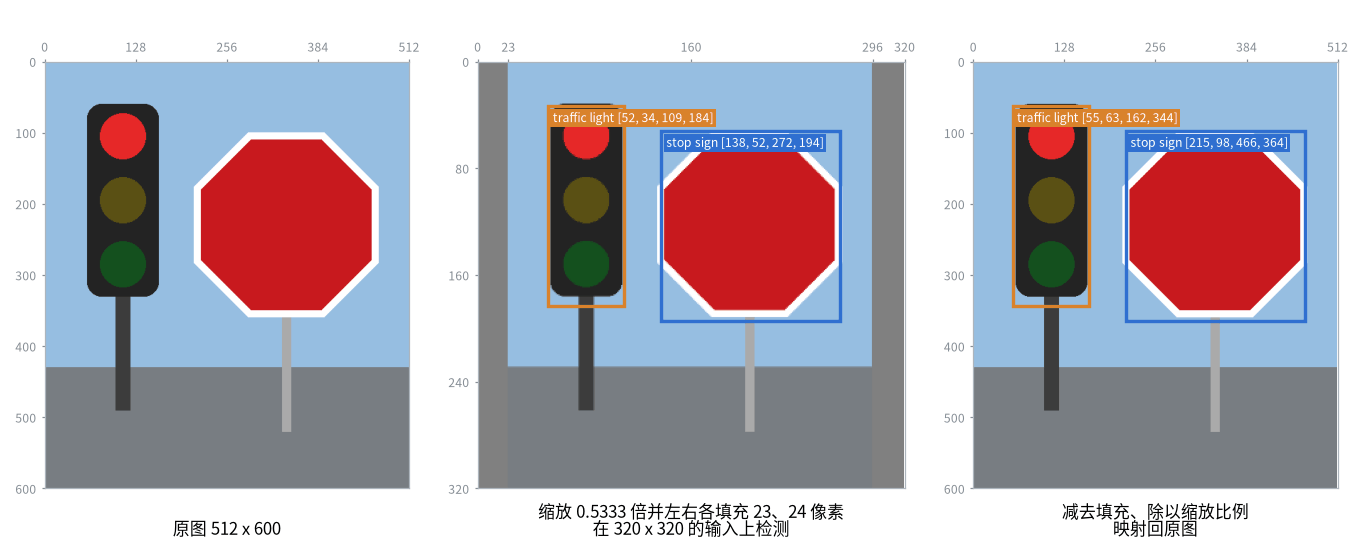
把同一张图像直接送入检测器,和先填充到 320x320 再检测并映射回原图,两种方式得到的框应当基本一致
1
2
3
4
5
6
7
8
9
10
11
12
13
14
15
16
17
18
19
20
21
22
23
import torch
from torchvision.models.detection import FasterRCNN_MobileNet_V3_Large_320_FPN_Weights, fasterrcnn_mobilenet_v3_large_320_fpn
from torchvision.transforms.functional import pil_to_tensor

from letterbox import letterbox, to_original
from scene import make_scene

weights = FasterRCNN_MobileNet_V3_Large_320_FPN_Weights.DEFAULT
model = fasterrcnn_mobilenet_v3_large_320_fpn(weights=weights, box_score_thresh=0.5)
model.eval()

image = make_scene()
x = pil_to_tensor(image).float() / 255      # (3, 600, 512)
resized, scale, pad = letterbox(x, 320)
print(resized.shape, round(scale, 4), pad)  # torch.Size([3, 320, 320]) 0.5333 (23, 0)

with torch.no_grad():
    direct = model([x])[0]['boxes']        # 直接在原图上检测
    boxes = model([resized])[0]['boxes']   # 在填充后的图像上检测,坐标属于 320x320 的图像

print(boxes.round())
print(to_original(boxes, scale, pad, x.shape[1:]).round())
print(direct.round())
1
2
3
4
5
6
7
torch.Size([3, 320, 320]) 0.5333 (23, 0)
tensor([[138.,  52., 272., 194.],
        [ 52.,  34., 109., 184.]])
tensor([[215.,  98., 466., 364.],
        [ 55.,  63., 162., 344.]])
tensor([[215.,  96., 471., 359.],
        [ 54.,  52., 165., 342.]])
三组结果依次为 320x320 输入上的框、映射回原图后的框、直接在原图上检测的框。后两组最多相差 11 个像素,是因为两次送入网络的图像本身不同
与相机参数配合
相机的内参是在原始分辨率下标定的,用检测框计算目标的方位角或进行测距之前,必须先把框映射回原图的坐标系(或者把内参按同样的缩放和平移进行换算)。视场角与焦距的关系见Field of View
1
2
3
4
5
6
7
8
9
10
11
import math

# 1920x1080 的相机,水平视场角 90 度,主点在图像中心
width, fov = 1920, 90
fx = width / 2 / math.tan(math.radians(fov) / 2)  # 以像素为单位的焦距
cx = width / 2

box = [600, 300, 1200, 900]  # 原图坐标系下的检测框
u = (box[0] + box[2]) / 2    # 框中心的横坐标
angle = math.degrees(math.atan((u - cx) / fx))
print(round(fx, 1), round(angle, 2))  # 960.0 -3.58,目标在光轴左侧 3.58 度
如果直接使用 640x640 输入上的坐标,框中心的横坐标是 300,按原图的内参会算出 -34.51 度,结果完全错误