PyTorch Deployment
整理 PyTorch 模型从训练到推理的过程,包括推理前的准备、导出 ONNX、ONNX Runtime 推理、预处理一致性、量化、耗时测量,以及 TensorRT 与 C++ 推理
深度学习系列:第 21 篇,共 22 篇
用 PyTorch 从搭建模型、训练、调试到部署的一组笔记。按下面的顺序阅读,后面的文章会直接引用前面讲过的内容
- PyTorch Deployment
- Model Compression
训练得到的是一份参数和一段 Python 代码,部署时往往要在没有 Python、没有 PyTorch 的环境里运行,例如机器人上的 C++ 程序。常见的做法是把模型导出为 ONNX,再交给 ONNX Runtime 或 TensorRT 执行。训练部分见PyTorch Training
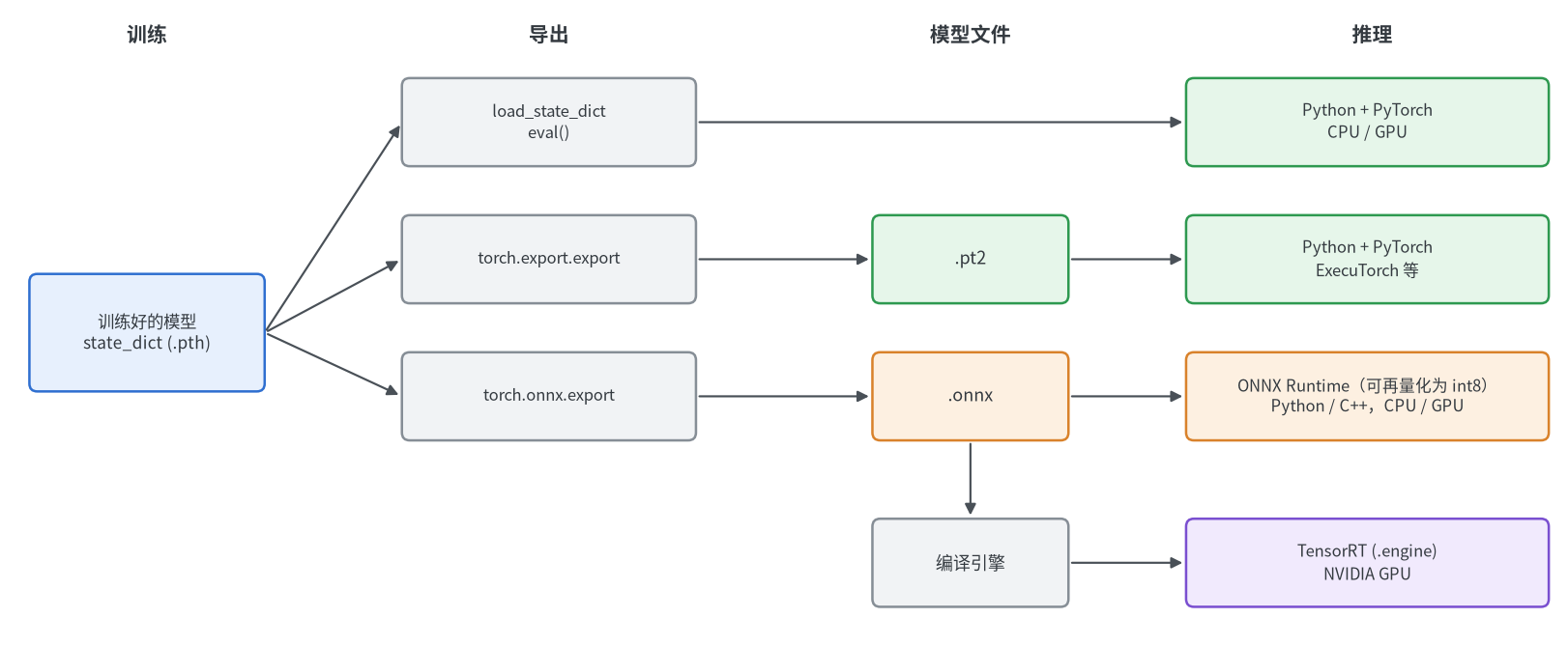
以下代码使用的模型是 torchvision 中带预训练权重的 ResNet-18
推理前的准备
评估模式
Dropout和BatchNorm在训练和推理时的行为不同(原理见Normalization and Regularization),推理前必须调用model.eval()切换到评估模式
1
2
3
4
5
6
7
8
9
10
11
12
13
14
15
16
17
18
19
import torch
from torchvision.models import ResNet18_Weights, resnet18

torch.manual_seed(0)
model = resnet18(weights=ResNet18_Weights.DEFAULT)
x = torch.randn(1, 3, 224, 224)
print(model.training)  # True,新建的模型默认处于训练模式

with torch.no_grad():
    model.eval()
    eval_out = model(x)
    print(torch.equal(model(x), eval_out))  # True,评估模式下同一输入的输出是确定的

    model.train()
    train_out = model(x)
    print((train_out - eval_out).abs().max().item())  # 6.59,训练模式下的输出完全不同

    model.eval()
    print((model(x) - eval_out).abs().max().item())   # 2.32,切回评估模式,输出也回不去了
训练模式下的每一次前向传播都会更新BatchNorm的统计量,即使在torch.no_grad()中也是如此。 忘记调用eval()不会报错,只是结果变差,而且统计量一旦被推理数据污染,再切回评估模式也无法恢复
关闭梯度
推理不需要反向传播,关闭梯度可以省去计算图占用的内存
| 方式 | 作用 | 得到的张量 |
|---|---|---|
torch.no_grad() | 不记录计算图 | 普通张量,之后仍可参与求导 |
torch.inference_mode() | 不记录计算图,同时省去版本计数等额外的记录 | 推理张量,不能再参与求导或被原地修改 |
1
2
3
4
5
6
7
8
9
10
11
12
13
14
15
16
17
18
19
20
21
22
23
24
25
26
27
28
29
import torch
from torchvision.models import resnet18

model = resnet18().eval()
x = torch.randn(1, 3, 224, 224)

y = model(x)
print(y.requires_grad)  # True,默认会记录计算图,白白占用内存

with torch.no_grad():
    y = model(x)
print(y.requires_grad, y.is_inference())  # False False

with torch.inference_mode():
    y = model(x)
print(y.requires_grad, y.is_inference())  # False True

try:
    y.add_(1)  # 推理模式下得到的张量,不能在推理模式之外原地修改
except RuntimeError as e:
    print(str(e).split(".")[0])  # Inplace update to inference tensor outside InferenceMode is not allowed


@torch.inference_mode()  # 也可以作为装饰器使用
def predict(x):
    return model(x).argmax(dim=1)


print(predict(x).shape)  # torch.Size([1])
纯推理的代码使用inference_mode();输出之后还要参与训练时使用no_grad(),例如用一个固定的模型为另一个模型生成训练目标
保存与加载
| 方式 | 保存的内容 | 加载时需要 |
|---|---|---|
| 保存参数 | 各层参数组成的字典 | 先用代码创建出相同结构的模型 |
| 保存整个模型 | 用pickle序列化的模型对象 | 能导入定义模型的类,且路径不变 |
1
2
3
4
5
6
7
8
9
10
11
12
13
14
15
16
17
18
19
20
21
22
23
24
25
26
import os
import pickle

import torch
from torchvision.models import ResNet18_Weights, resnet18

model = resnet18(weights=ResNet18_Weights.DEFAULT).eval()

# 方式一:只保存参数,加载时需要先用代码创建出相同结构的模型
torch.save(model.state_dict(), "resnet18.pth")
print(f"{os.path.getsize('resnet18.pth') / 1e6:.1f} MB")  # 46.8 MB

model = resnet18()
state_dict = torch.load("resnet18.pth", map_location="cpu")
print(model.load_state_dict(state_dict))  # <All keys matched successfully>
model.eval()

# 方式二:保存整个模型对象
torch.save(model, "resnet18_full.pth")
try:
    torch.load("resnet18_full.pth")
except pickle.UnpicklingError as e:
    print(str(e).split("\n")[0][:30])  # Weights only load failed. This

model = torch.load("resnet18_full.pth", weights_only=False)  # 只对来源可信的文件这样做
print(type(model).__name__)  # ResNet
torch.load默认只允许加载张量、字典等基本类型,加载整个模型对象会报错Weights only load failed,需要显式传入weights_only=False。这样做会执行文件中的任意代码,不要用它加载来历不明的文件,详见PyTorch Checkpoints and Reproducibilitymap_location="cpu"把在 GPU 上保存的参数加载到 CPU,在没有 GPU 的机器上加载时必须指定- 推荐只保存参数。保存整个模型时,文件里记录的是类的导入路径,代码一旦重构就无法加载
导出方式对比
| 方式 | 文件 | 运行时需要 | 目前的状态 |
|---|---|---|---|
| 参数加 Python 代码 | .pth | PyTorch 和定义模型的代码 | 推荐的保存方式 |
| TorchScript | .pt | PyTorch 或 libtorch,不需要模型代码 | 仍可使用,调用时给出弃用警告 |
torch.export | .pt2 | PyTorch,不需要模型代码 | 取代 TorchScript,也是导出 ONNX 的基础 |
| ONNX | .onnx | ONNX Runtime、TensorRT 等,不需要 PyTorch | 默认使用基于torch.export的新导出器 |
离开 Python 环境部署时选择 ONNX。torch.export把模型转换为一张不依赖 Python 代码的计算图,新的 ONNX 导出器就是先调用它,再把图翻译为 ONNX
1
2
3
4
5
6
7
8
9
10
11
12
13
14
15
16
17
18
19
20
21
22
23
24
25
26
27
28
29
import warnings

import torch
from torchvision.models import ResNet18_Weights, resnet18

model = resnet18(weights=ResNet18_Weights.DEFAULT).eval()
x = torch.randn(1, 3, 224, 224)

# TorchScript:仍然可用,但会给出弃用警告
with warnings.catch_warnings(record=True) as caught:
    warnings.simplefilter("always")
    traced = torch.jit.trace(model, x)
print(caught[0].category.__name__, caught[0].message)
# FutureWarning `torch.jit.trace` is deprecated. Please switch to `torch.compile` or `torch.export`.

# torch.export:导出为ExportedProgram,第0维标记为动态
batch = torch.export.Dim("batch")
try:
    torch.export.export(model, (x,), dynamic_shapes={"x": {0: batch}})
except Exception as e:
    print(type(e).__name__)  # UserError,示例输入的批大小为1时,这一维会被当成常量

program = torch.export.export(model, (torch.randn(2, 3, 224, 224),), dynamic_shapes={"x": {0: batch}})
torch.export.save(program, "resnet18.pt2")

loaded = torch.export.load("resnet18.pt2").module()
print(loaded(torch.randn(8, 3, 224, 224)).shape)  # torch.Size([8, 1000])
with torch.no_grad():
    print(torch.allclose(loaded(x), model(x), atol=1e-5))  # True
需要动态批大小时,示例输入的批大小不要取 1。 torch.export会把大小为 0 或 1 的维度当成常量,直接导出时报错You marked batch as dynamic but your code specialized it to be a constant (1),把示例输入的批大小改为 2 即可,导出后的模型同样可以接收批大小为 1 的输入
导出 ONNX
导出与检查
1
2
3
4
5
6
7
8
9
10
11
12
13
14
15
16
17
18
19
20
21
22
23
24
25
26
27
28
29
30
import os

import onnx
import torch
from torchvision.models import ResNet18_Weights, resnet18

model = resnet18(weights=ResNet18_Weights.DEFAULT).eval()
example = torch.randn(2, 3, 224, 224)

torch.onnx.export(
    model,
    (example,),
    "resnet18.onnx",
    input_names=["input"],
    output_names=["logits"],
    dynamic_shapes={"x": {0: "batch"}},  # 键是forward的参数名,第0维为动态
    external_data=False,                 # 权重写入同一个文件
    verbose=False,                       # 不打印导出过程
)

onnx_model = onnx.load("resnet18.onnx")
onnx.checker.check_model(onnx_model)  # 模型不合法时抛出异常

print(f"{os.path.getsize('resnet18.onnx') / 1e6:.1f} MB")  # 46.8 MB
print(onnx_model.opset_import[0].version)                  # 20
for tensor in list(onnx_model.graph.input) + list(onnx_model.graph.output):
    shape = [d.dim_param or d.dim_value for d in tensor.type.tensor_type.shape.dim]
    print(tensor.name, shape)
# input ['batch', 3, 224, 224]
# logits ['batch', 1000]
导出前同样要先调用model.eval()。导出器按示例输入执行一遍模型并记录下经过的运算,forward中如果有依赖输入数值的if,例如if x.sum() > 0,新导出器会报错TorchExportError,需要改写模型;旧导出器不报错,只给出一条TracerWarning,然后把示例输入走过的那一条分支固定下来,换一个输入结果就可能是错的
主要参数
| 参数 | 默认值 | 说明 |
|---|---|---|
input_namesoutput_names | None | 输入和输出的名字,推理时按名字传入数据 |
dynamic_shapes | None | 哪些维度的大小可变,不指定时所有维度固定为示例输入的形状 |
opset_version | None | 算子集版本,不指定时实际得到的是 20 |
external_data | True | 权重是否单独存放在.onnx.data文件中 |
dynamo | True | 使用基于torch.export的新导出器,False为旧导出器 |
verify | False | 导出后用 ONNX Runtime 运行一遍,与 PyTorch 的输出比较 |
verbose | None | 是否打印导出过程,默认打印 |
以下几点都是实际运行得到的结果
- 不指定
input_names和output_names时,名字分别是forward的参数名x和最后一个运算的名字linear,后者会随模型改动而变化,部署代码中要用到名字,最好显式指定 - 不指定
dynamic_shapes时批大小固定,用批大小 1 导出的模型传入 4 张图像,ONNX Runtime 报错Got invalid dimensions for input: x ... Got: 4 Expected: 1 external_data默认为True,导出的resnet18.onnx只有 0.1 MB,权重在旁边的resnet18.onnx.data中,两个文件必须放在一起。模型小于 2 GB 时设为False更省事- 新导出器支持的最低算子集版本为 18,指定
opset_version=17时得到的仍然是 18,只在日志中给出提示 - 旧的
dynamic_axes参数仍然可用,但会给出警告,建议改用dynamic_shapes dynamo=False使用基于 TorchScript 的旧导出器,会给出弃用警告,它可以导出opset_version=17的模型,只在推理引擎不支持较新的算子集时使用
ONNX Runtime 推理
推理与结果对比
ONNX Runtime 的输入和输出都是 NumPy 数组,推理时不需要 PyTorch。导出之后要做的第一件事,是用相同的输入比较它和 PyTorch 的输出
1
2
3
4
5
6
7
8
9
10
11
12
13
14
15
16
17
18
19
20
21
22
23
24
25
26
27
28
29
30
import numpy as np
import onnxruntime as ort
import torch
from torchvision.models import ResNet18_Weights, resnet18

print(ort.get_available_providers())
# ['TensorrtExecutionProvider', 'CUDAExecutionProvider', 'CPUExecutionProvider']

session = ort.InferenceSession("resnet18.onnx", providers=["CPUExecutionProvider"])
for tensor in session.get_inputs() + session.get_outputs():
    print(tensor.name, tensor.shape, tensor.type)
# input ['batch', 3, 224, 224] tensor(float)
# logits ['batch', 1000] tensor(float)

model = resnet18(weights=ResNet18_Weights.DEFAULT).eval()
rng = np.random.default_rng(0)
for batch_size in (1, 4):
    x = rng.standard_normal((batch_size, 3, 224, 224), dtype=np.float32)
    onnx_out = session.run(["logits"], {"input": x})[0]  # 输入输出都是numpy数组
    with torch.inference_mode():
        torch_out = model(torch.from_numpy(x)).numpy()
    print(onnx_out.shape, np.abs(onnx_out - torch_out).max(), np.allclose(onnx_out, torch_out, atol=1e-4))
# (1, 1000) 3.8146973e-06 True
# (4, 1000) 4.2915344e-06 True

try:
    session.run(None, {"input": x.astype(np.float64)})  # numpy默认的float64不会被自动转换
except Exception as e:
    print(type(e).__name__, str(e).split(": ", 3)[-1])
# InvalidArgument Unexpected input data type. Actual: (tensor(double)) , expected: (tensor(float))
- 两边的输出相差在$10^{-6}$量级,这是浮点运算顺序不同造成的正常误差。比较时用
np.allclose并给出容差,不要用== session.run的第一个参数是需要的输出名字的列表,None表示全部输出- 输入的数据类型必须与模型一致。NumPy 默认是
float64,图像是uint8,都需要先转换为float32
执行提供方
providers指定用什么设备执行,按列表中的顺序依次尝试,某个算子不被前面的提供方支持时交给后面的执行
| 提供方 | 设备 | 需要安装 |
|---|---|---|
CPUExecutionProvider | CPU | onnxruntime |
CUDAExecutionProvider | NVIDIA GPU | onnxruntime-gpu,以及 CUDA 和 cuDNN |
TensorrtExecutionProvider | NVIDIA GPU | onnxruntime-gpu,以及 TensorRT |
get_available_providers()列出的是安装包中包含的提供方,不代表它们一定能用。下面的代码在装有onnxruntime-gpu的环境中运行
1
2
3
4
5
6
7
8
9
10
11
12
13
14
15
16
17
import numpy as np
import onnxruntime as ort

providers = ["CUDAExecutionProvider", "CPUExecutionProvider"]

session = ort.InferenceSession("resnet18.onnx", providers=providers)
print(session.get_providers())  # ['CPUExecutionProvider'],没有找到CUDA的动态库,退回了CPU

ort.preload_dlls()  # 先加载随pip安装的CUDA和cuDNN动态库
session = ort.InferenceSession("resnet18.onnx", providers=providers)
print(session.get_providers())  # ['CUDAExecutionProvider', 'CPUExecutionProvider']

x = np.random.default_rng(0).standard_normal((4, 3, 224, 224), dtype=np.float32)
cpu_session = ort.InferenceSession("resnet18.onnx", providers=["CPUExecutionProvider"])
gpu_out = session.run(None, {"input": x})[0]
cpu_out = cpu_session.run(None, {"input": x})[0]
print(np.abs(gpu_out - cpu_out).max(), (gpu_out.argmax(axis=1) == cpu_out.argmax(axis=1)).all())
1
2
3
['CPUExecutionProvider']
['CUDAExecutionProvider', 'CPUExecutionProvider']
0.0043742657 True
- GPU 提供方创建失败时不会抛出异常,而是退回 CPU 继续运行。 第一次创建会话时,
onnxruntime找不到随 pip 安装的 CUDA 和 cuDNN 动态库,只在日志中打印一条Failed to create CUDAExecutionProvider,程序照常运行,只是慢了一个数量级 - 创建会话之前调用
ort.preload_dlls()把这些动态库加载进来就可以了。在import onnxruntime之前先import torch也有同样的效果,因为 PyTorch 已经加载了它们 - 创建会话之后一定要打印
session.get_providers(),确认实际生效的提供方 - GPU 与 CPU 的输出相差约 0.004,比 CPU 上 ONNX Runtime 与 PyTorch 之间的$10^{-6}$大得多,预测的类别相同。GPU 上卷积的实现不同,比较时容差要相应放宽
onnxruntime和onnxruntime-gpu不能同时安装。GPU 版对 CUDA 和 cuDNN 的版本有要求,放在容器里最省事,容器中使用显卡的配置见Docker Configuration
预处理一致性
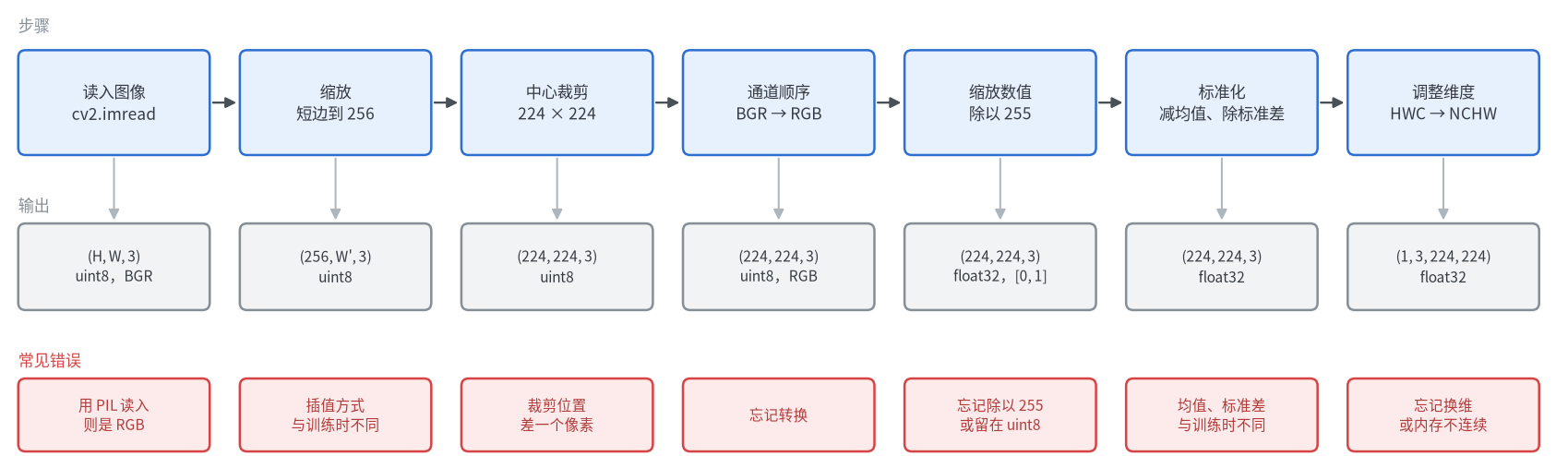
模型导出正确、数值对比也通过,部署后的效果却明显变差,原因大多在预处理:推理时送入模型的张量,与训练时的不是同一种
用 OpenCV 实现预处理
训练时用的是 torchvision 的预处理:短边缩放到 256,中心裁剪 224,除以 255,再按通道减均值、除标准差。部署端通常只有 OpenCV 和 NumPy,需要把同样的步骤重新实现一遍
1
2
3
4
5
6
7
8
9
10
11
12
13
14
15
16
17
18
19
20
21
22
23
24
25
26
27
28
29
30
31
32
33
34
35
36
37
38
39
40
41
42
import cv2
import numpy as np
from PIL import Image

MEAN = np.array([0.485, 0.456, 0.406], dtype=np.float32)
STD = np.array([0.229, 0.224, 0.225], dtype=np.float32)


def resize_area(image, size):
    return cv2.resize(image, size, interpolation=cv2.INTER_AREA)


def resize_linear(image, size):
    return cv2.resize(image, size, interpolation=cv2.INTER_LINEAR)


def resize_pil(image, size):
    return np.asarray(Image.fromarray(image).resize(size, Image.BILINEAR))


def preprocess(image, resize=resize_area):
    """image为cv2.imread读入的图像:形状(H, W, 3)、uint8、通道顺序BGR"""
    h, w = image.shape[:2]
    # 短边缩放到256,长边按比例缩放并向下取整,与torchvision一致
    nh, nw = (256, int(256 * w / h)) if h <= w else (int(256 * h / w), 256)
    image = resize(image, (nw, nh))                 # 尺寸的顺序是(宽, 高)
    top, left = round((nh - 224) / 2), round((nw - 224) / 2)
    image = image[top:top + 224, left:left + 224]   # 中心裁剪
    image = cv2.cvtColor(image, cv2.COLOR_BGR2RGB)  # BGR -> RGB
    x = image.astype(np.float32) / 255.0            # uint8 [0, 255] -> float32 [0, 1]
    x = (x - MEAN) / STD                            # 按通道标准化,此时通道在最后一维
    x = x.transpose(2, 0, 1)[None]                  # (H, W, C) -> (1, C, H, W)
    return np.ascontiguousarray(x)                  # transpose之后内存不连续,转为连续


image = cv2.imread("test.jpg")
print(image.shape, image.dtype)  # (427, 640, 3) uint8

x = preprocess(image)
print(x.shape, x.dtype)          # (1, 3, 224, 224) float32

np.savez("inputs.npz", pil=preprocess(image, resize_pil), area=x, linear=preprocess(image, resize_linear))
test.jpg是任意一张图像,这里用的是 scikit-learn 自带的示例图片china.jpg。最后一行把送入模型的张量保存下来,用于和训练端比较。这是排查预处理问题最直接的办法:两边各保存一份,逐元素比较
与训练时的预处理比较
1
2
3
4
5
6
7
8
9
10
11
12
13
14
15
16
17
18
19
20
21
22
23
24
25
26
27
28
import numpy as np
import torch
from PIL import Image
from torchvision.models import ResNet18_Weights, resnet18

weights = ResNet18_Weights.DEFAULT
model = resnet18(weights=weights).eval()
categories = weights.meta["categories"]

# 训练和验证时使用的预处理
reference = weights.transforms()(Image.open("test.jpg")).unsqueeze(0)

mean = torch.tensor([0.485, 0.456, 0.406]).view(1, 3, 1, 1)
std = torch.tensor([0.229, 0.224, 0.225]).view(1, 3, 1, 1)
inputs = {k: torch.from_numpy(v) for k, v in np.load("inputs.npz").items()}
raw = inputs["area"] * std + mean                      # 还原为标准化之前的[0, 1]
inputs["no_swap"] = (raw.flip(1) - mean) / std         # 忘记BGR -> RGB
inputs["no_normalize"] = raw                           # 只除以255,没有标准化
inputs["no_scale"] = raw * 255                         # 没有除以255,也没有标准化

with torch.inference_mode():
    target = model(reference).softmax(dim=1).argmax().item()
    print(f"{'reference':<13}{categories[target]:<12}{model(reference).softmax(dim=1)[0, target].item():.3f}")
    for name, x in inputs.items():
        prob = model(x).softmax(dim=1)[0]
        diff = (x - reference).abs()
        print(f"{name:<13}{categories[prob.argmax().item()]:<12}{prob[target].item():.3f}  "
              f"max={diff.max().item():.4f}  mean={diff.mean().item():.4f}")
1
2
3
4
5
6
7
reference    bell cote   0.536
pil          bell cote   0.536  max=0.0000  mean=0.0000
area         bell cote   0.490  max=0.5137  mean=0.0318
linear       bell cote   0.562  max=1.3700  mean=0.0759
no_swap      boathouse   0.082  max=3.2593  mean=0.3478
no_normalize palace      0.255  max=2.1047  mean=0.9876
no_scale     plunger     0.000  max=252.8367  mean=144.3105
| 输入 | 与训练端的差别 | 结果 |
|---|---|---|
pil | 无,缩放也使用 PIL | 与训练端完全相同 |
area | 缩放使用cv2.INTER_AREA | 类别相同,概率从 0.536 变为 0.490 |
linear | 缩放使用cv2.INTER_LINEAR | 类别相同,张量的平均差值是area的两倍多 |
no_swap | 没有把 BGR 转为 RGB | 类别错误,正确类别的概率降到 0.082 |
no_normalize | 没有减均值、除标准差 | 类别错误 |
no_scale | 没有除以 255 | 类别错误,概率接近 1,错得很自信 |
- 通道顺序、数值范围、标准化这几项弄错时不会报错,模型照样给出一个结果,只是结果是错的
- 除了缩放,其余步骤都可以做到与训练端完全相同。
pil一行说明裁剪、通道、标准化、维度的实现没有问题 - 缩放是唯一无法逐位对齐的步骤。 torchvision 缩小图像时带有抗锯齿,
cv2.INTER_LINEAR没有,缩小图像时cv2.INTER_AREA更接近。这个差别不会让结果全错,但会让准确率略有下降,部署后应当用部署端的预处理在验证集上重新评估一次 - 如果训练时就能确定部署端使用 OpenCV,直接在训练的数据集中也用 OpenCV 读图和缩放,可以消除这一差别
- 裁剪位置的取整方式也要一致,C++ 部分有一个差一个像素导致预测类别改变的例子
量化
量化把 32 位浮点数表示的权重和中间结果换成 8 位整数,模型大小约为原来的四分之一,在 CPU 上的计算也可能更快,代价是精度略有下降。这里只涉及训练后量化,剪枝、蒸馏和量化感知训练见Model Compression
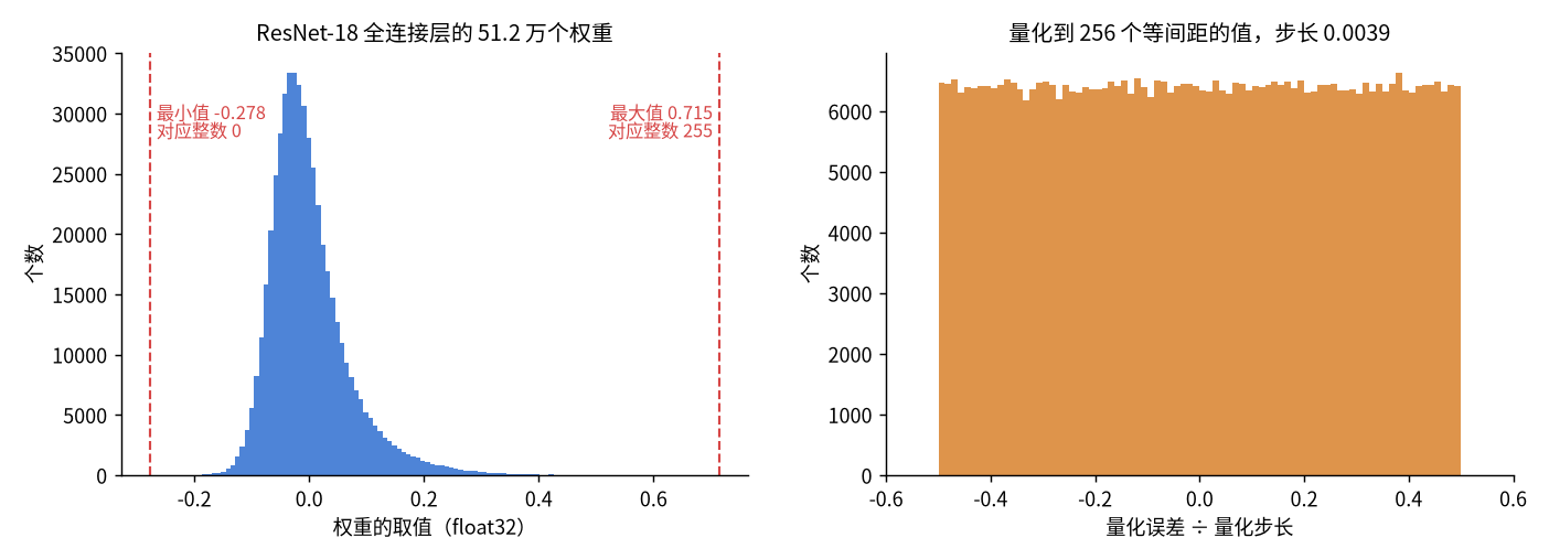
把权重的最小值到最大值之间均匀分成 255 份,每个权重取最近的一个刻度,误差不超过半个步长
| 方式 | 需要的数据 | 做法 |
|---|---|---|
| 动态量化 | 不需要 | 权重提前量化,中间结果的范围在推理时临时统计 |
| 静态量化 | 少量校准数据 | 用校准数据提前统计好中间结果的范围,推理时全程使用整数 |
| 量化感知训练 | 训练数据和训练过程 | 训练时模拟量化带来的误差,让模型去适应,精度损失最小 |
PyTorch 自带的量化
1
2
3
4
5
6
7
8
9
10
11
12
13
14
15
16
17
18
import os
import warnings

import torch
from torch import nn
from torchvision.models import ResNet18_Weights, resnet18

model = resnet18(weights=ResNet18_Weights.DEFAULT).eval()

with warnings.catch_warnings(record=True) as caught:
    warnings.simplefilter("always")
    quantized = torch.ao.quantization.quantize_dynamic(model, {nn.Linear}, dtype=torch.qint8)
print(sorted({w.category.__name__ for w in caught}))  # ['DeprecationWarning', 'UserWarning']
print(quantized.fc)     # DynamicQuantizedLinear(in_features=512, out_features=1000, dtype=torch.qint8, ...)
print(quantized.conv1)  # Conv2d(3, 64, kernel_size=(7, 7), ...),卷积层没有被量化

torch.save(quantized.state_dict(), "resnet18_quantized.pth")
print(f"{os.path.getsize('resnet18_quantized.pth') / 1e6:.1f} MB")  # 45.3 MB,原来是46.8 MB
torch.ao.quantization目前仍然可以运行,但调用时给出弃用警告,提示迁移到单独的torchao库- PyTorch 的动态量化只支持
nn.Linear、nn.LSTM等层,不支持卷积。ResNet-18 的参数几乎都在卷积层中,量化后只从 46.8 MB 减小到 45.3 MB - 量化后的模型只能在 CPU 上运行
因此对于卷积网络,更实用的做法是在导出 ONNX 之后用 ONNX Runtime 的量化工具
ONNX Runtime 量化
1
2
3
4
5
6
7
8
9
10
11
12
13
14
15
16
17
18
19
20
21
22
23
24
25
26
27
28
29
30
31
32
33
34
35
36
37
38
39
40
41
42
43
44
45
46
47
48
49
50
51
52
53
54
55
56
57
58
import os

import numpy as np
import onnxruntime as ort
import torch
from onnxruntime.quantization import CalibrationDataReader, QuantFormat, QuantType, quantize_dynamic, quantize_static
from onnxruntime.quantization.shape_inference import quant_pre_process
from PIL import Image
from sklearn.datasets import load_sample_images
from torchvision.transforms import v2

torch.manual_seed(0)

# 示例只有两张图片,用随机裁剪得到校准数据和测试数据;实际应使用几百张训练集中的图片
images = [Image.fromarray(image) for image in load_sample_images().images]
transform = v2.Compose([
    v2.RandomResizedCrop(224, scale=(0.3, 1.0)),
    v2.ToImage(),
    v2.ToDtype(torch.float32, scale=True),
    v2.Normalize([0.485, 0.456, 0.406], [0.229, 0.224, 0.225]),
])


def make_batch(n):
    return torch.stack([transform(images[i % 2]) for i in range(n)]).numpy()


class Reader(CalibrationDataReader):
    """每次返回一个批次的输入,返回None表示校准数据已经用完"""

    def __init__(self, data, batch_size=8):
        self.batches = iter(np.split(data, len(data) // batch_size))

    def get_next(self):
        batch = next(self.batches, None)
        return None if batch is None else {"input": batch}


quant_pre_process("resnet18.onnx", "resnet18_pre.onnx")  # 形状推断与图优化,量化前先做一次

quantize_dynamic("resnet18_pre.onnx", "resnet18_dynamic.onnx", weight_type=QuantType.QUInt8)
quantize_static(
    "resnet18_pre.onnx",
    "resnet18_static.onnx",
    Reader(make_batch(64)),
    quant_format=QuantFormat.QDQ,
    per_channel=True,  # 卷积的每个输出通道使用各自的缩放系数
)

test = make_batch(200)
reference = None
for name in ("resnet18", "resnet18_dynamic", "resnet18_static"):
    session = ort.InferenceSession(f"{name}.onnx", providers=["CPUExecutionProvider"])
    predictions = session.run(None, {"input": test})[0].argmax(axis=1)
    if reference is None:
        reference = predictions
    size = os.path.getsize(f"{name}.onnx") / 1e6
    print(f"{name:<18}{size:5.1f} MB  与原模型预测相同的比例 {(predictions == reference).mean():.3f}")
1
2
3
resnet18           46.8 MB  与原模型预测相同的比例 1.000
resnet18_dynamic   11.8 MB  与原模型预测相同的比例 0.950
resnet18_static    11.9 MB  与原模型预测相同的比例 0.945
- 两种量化都把模型从 46.8 MB 减小到约 11.8 MB,在 200 张随机裁剪的图像上,约 95% 的预测与原模型相同。这只是一个粗略的参考,真正的精度损失要在验证集上评估
- 不要跳过
quant_pre_process。 直接对新导出器导出的模型调用quantize_dynamic会报错ShapeInferenceError: Inferred shape and existing shape differ in dimension 0: (512) vs (1000),先做预处理就没有问题 - 校准数据必须经过与推理时完全相同的预处理,否则统计出的数值范围是错的
- 量化能否加快推理取决于 CPU 的指令集和推理引擎,必须实际测量,见下一节
量化感知训练需要重新训练,只在静态量化的精度损失无法接受时才使用,这里不展开
性能测量
测量方法
| 要点 | 原因 |
|---|---|
| 预热 | 前几次调用包含内存分配、算法选择等一次性开销,不能计入 |
| 多次重复取中位数 | 单次耗时受系统中其他任务影响,平均值容易被个别很慢的调用拉高 |
| 固定线程数 | CPU 推理的耗时与线程数直接相关,不固定就无法比较 |
| GPU 同步 | GPU 上的计算是异步的,计时结束前要调用torch.cuda.synchronize() |
| 使用真实的输入 | 输入的形状和批大小要与实际使用时相同 |
1
2
3
4
5
6
7
8
9
10
11
12
13
14
15
16
17
18
19
20
21
22
23
24
25
26
27
28
29
30
31
32
33
34
35
36
37
38
39
40
41
42
43
44
45
46
47
48
49
50
51
52
53
54
55
56
57
58
59
import copy
import time

import numpy as np
import onnxruntime as ort
import torch
from torchvision.models import ResNet18_Weights, resnet18

THREADS = 4
torch.set_num_threads(THREADS)


def benchmark(fn, warmup=20, repeat=100):
    """返回单次调用耗时的中位数,单位为毫秒"""
    for _ in range(warmup):  # 预热:前几次调用包含内存分配、算法选择等一次性开销
        fn()
    times = []
    for _ in range(repeat):
        start = time.perf_counter()
        fn()
        times.append(time.perf_counter() - start)
    return float(np.median(times)) * 1000


def torch_runner(model, x, device):
    model, x = copy.deepcopy(model).to(device), x.to(device)  # 模块的to()是原地操作,先复制一份

    def run():
        with torch.inference_mode():
            model(x)
        if device == "cuda":
            torch.cuda.synchronize()  # GPU上的计算是异步的,等它算完再停止计时

    return run


def onnx_runner(path, x, provider="CPUExecutionProvider"):
    options = ort.SessionOptions()
    options.intra_op_num_threads = THREADS
    session = ort.InferenceSession(path, options, providers=[provider])
    return lambda: session.run(None, {"input": x})


results = {}
for batch_size in (1, 8):
    x = torch.randn(batch_size, 3, 224, 224)
    model = resnet18(weights=ResNet18_Weights.DEFAULT).eval()
    runners = {
        "PyTorch CPU": torch_runner(model, x, "cpu"),
        "ONNX Runtime CPU": onnx_runner("resnet18.onnx", x.numpy()),
        "ONNX Runtime CPU 动态量化": onnx_runner("resnet18_dynamic.onnx", x.numpy()),
        "ONNX Runtime CPU 静态量化": onnx_runner("resnet18_static.onnx", x.numpy()),
    }
    if torch.cuda.is_available():
        runners["PyTorch GPU"] = torch_runner(model, x, "cuda")
        runners["ONNX Runtime GPU"] = onnx_runner("resnet18.onnx", x.numpy(), "CUDAExecutionProvider")
    for name, run in runners.items():
        results[name, batch_size] = benchmark(run)
        print(f"{name:<24} batch={batch_size}  {results[name, batch_size]:7.2f} ms")
脚本中先导入了torch,所以 ONNX Runtime 的 GPU 提供方可以直接创建,不需要再调用ort.preload_dlls()
nn.Module的to()会原地移动模型本身,张量的to()则返回一个新的张量。同一个模型既要在 CPU 上测又要在 GPU 上测时,要先复制一份,否则报错Input type (torch.FloatTensor) and weight type (torch.cuda.FloatTensor) should be the same
测量结果
测量使用的机器为 Intel Core Ultra 9 285K、GeForce RTX 5090 D(32 GB 显存)、64 GB 内存,CPU 推理固定 4 个线程。下表为上面脚本一次运行的输出,TensorRT 一行来自下一节的脚本,单位为毫秒。同样的测量又重复了 6 遍,各项与表中数值的相差大多在 5% 以内,波动最大的是 PyTorch CPU 批大小 8 一项,在 58 到 64 毫秒之间
| 推理方式 | 批大小 1 | 批大小 8 |
|---|---|---|
| PyTorch CPU | 9.16 | 64.49 |
| ONNX Runtime CPU | 5.97 | 46.76 |
| ONNX Runtime CPU 动态量化 | 5.06 | 39.30 |
| ONNX Runtime CPU 静态量化 | 6.83 | 48.60 |
| PyTorch GPU | 0.66 | 0.91 |
| ONNX Runtime GPU | 0.57 | 1.11 |
| TensorRT | 0.43 | 0.77 |
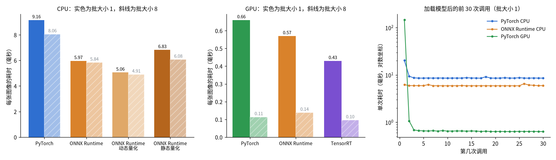
- CPU 上 ONNX Runtime 比 PyTorch 快,批大小为 1 时耗时约为后者的三分之二
- 量化的效果因方式而异。 动态量化是 CPU 上最快的,批大小为 1 时比浮点模型快约 15%;静态量化反而比浮点模型慢。量化一定能减小模型,但不一定能加快推理,必须在目标设备上实测
- GPU 上三种方式的耗时都在 1 毫秒上下,比 CPU 快一个数量级,其中 TensorRT 最快
- GPU 上批大小从 1 增加到 8,PyTorch 的总耗时只从 0.66 毫秒增加到 0.91 毫秒,平均每张图像 0.11 毫秒,能攒批时尽量攒批。CPU 上攒批的收益很小,每张图像从 9.2 毫秒降到 8.1 毫秒
- ONNX Runtime GPU 的输入是 CPU 上的 NumPy 数组,每次调用都包含把数据拷贝到 GPU 的时间;PyTorch GPU 和 TensorRT 的输入已经在 GPU 上。批大小为 8 时 ONNX Runtime GPU 比 PyTorch GPU 慢,与此有关
- GPU 的第一次调用用了 147 毫秒,之后稳定在 0.7 毫秒左右,相差 200 多倍;PyTorch CPU 的第一次调用是 20 毫秒,之后是 8.7 毫秒。这就是必须预热的原因
- 这个模型在 GPU 上不调用
torch.cuda.synchronize()测到的中位数是 0.54 毫秒,调用后是 0.64 毫秒,少算了约 15%。模型越大、批越大,不同步时测到的越可能只是把任务提交给 GPU 的时间 - 这里测的只是模型的前向计算。实际部署中读图、预处理、后处理的耗时常常与模型相当,在 GPU 上甚至远超模型本身,应当对整条流程计时
TensorRT 与 C++ 推理
TensorRT
TensorRT 是 NVIDIA 的推理引擎,针对具体的显卡把 ONNX 模型编译成引擎文件,通常是 NVIDIA GPU 上最快的推理方式。下面用它的 Python 接口(pip 包tensorrt)编译引擎,并直接用 PyTorch 在 GPU 上的张量作为输入和输出
1
2
3
4
5
6
7
8
9
10
11
12
13
14
15
16
17
18
19
20
21
22
23
24
25
26
27
28
29
30
31
32
33
34
35
36
37
38
39
40
41
42
43
44
45
46
47
48
49
50
51
52
53
54
55
56
57
import time

import numpy as np
import tensorrt as trt
import torch
from torchvision.models import ResNet18_Weights, resnet18

logger = trt.Logger(trt.Logger.WARNING)

# 1. 把ONNX模型编译为引擎
builder = trt.Builder(logger)
network = builder.create_network(0)
parser = trt.OnnxParser(network, logger)
assert parser.parse_from_file("resnet18.onnx"), [parser.get_error(i) for i in range(parser.num_errors)]

config = builder.create_builder_config()
profile = builder.create_optimization_profile()  # 动态批大小:最小、最常用、最大的形状
profile.set_shape("input", (1, 3, 224, 224), (1, 3, 224, 224), (8, 3, 224, 224))
config.add_optimization_profile(profile)

start = time.perf_counter()
serialized = builder.build_serialized_network(network, config)
print(f"编译耗时 {time.perf_counter() - start:.1f} 秒")
with open("resnet18.engine", "wb") as f:
    f.write(serialized)

# 2. 加载引擎并推理,输入和输出直接使用GPU上的张量
runtime = trt.Runtime(logger)
engine = runtime.deserialize_cuda_engine(serialized)
context = engine.create_execution_context()


def infer(x):
    y = torch.empty(x.size(0), 1000, device="cuda")
    context.set_input_shape("input", tuple(x.shape))
    context.set_tensor_address("input", x.data_ptr())
    context.set_tensor_address("logits", y.data_ptr())
    context.execute_async_v3(torch.cuda.current_stream().cuda_stream)
    torch.cuda.synchronize()
    return y


model = resnet18(weights=ResNet18_Weights.DEFAULT).eval().cuda()
for batch_size in (1, 8):
    x = torch.randn(batch_size, 3, 224, 224, device="cuda")
    with torch.inference_mode():
        expected = model(x)
    print(batch_size, float((infer(x) - expected).abs().max()))  # 与PyTorch输出的最大差异

    for _ in range(20):
        infer(x)
    times = []
    for _ in range(100):
        start = time.perf_counter()
        infer(x)
        times.append(time.perf_counter() - start)
    print(f"TensorRT batch={batch_size}  {np.median(times) * 1000:.2f} ms")
1
2
3
4
5
编译耗时 4.6 秒
1 0.005790889263153076
TensorRT batch=1  0.43 ms
8 0.008614301681518555
TensorRT batch=8  0.77 ms
set_shape和set_tensor_address中的input、logits就是导出 ONNX 时指定的名字- 模型的批大小是动态的,必须通过优化配置给出最小、最常用、最大三个形状,引擎针对最常用的形状优化,推理时的形状不能超出范围
set_tensor_address只传入地址,不检查大小和数据类型,输出张量要按正确的形状提前分配好,并且在推理结束前保持有效- 与 PyTorch 的输出相差在 0.01 以内,和 ONNX Runtime GPU 的误差在同一量级
- 引擎文件与 TensorRT 版本、显卡型号绑定,换一台机器要重新编译,不能把引擎文件当作模型分发,应当分发 ONNX 文件
随 TensorRT 的系统安装包提供的命令行工具trtexec可以不写代码完成同样的事情。下面的命令没有在本文中实际运行
1
2
3
4
5
6
7
8
# 把ONNX模型编译为引擎文件
trtexec --onnx=resnet18.onnx --saveEngine=resnet18.engine \
    --minShapes=input:1x3x224x224 \
    --optShapes=input:1x3x224x224 \
    --maxShapes=input:8x3x224x224

# 加载引擎文件并测量耗时
trtexec --loadEngine=resnet18.engine --shapes=input:1x3x224x224
C++ 推理
ONNX Runtime 提供 C++ 接口,从发布页下载对应平台的压缩包,解压后包含头文件和动态库。下面的程序用 OpenCV 读图并做预处理,再用 ONNX Runtime 推理,预处理与前面 Python 中的preprocess逐步对应
1
2
3
4
5
6
7
8
9
10
11
12
13
14
15
16
17
18
19
20
21
22
23
24
25
26
27
28
29
30
31
32
33
34
35
36
37
38
39
40
41
42
43
44
45
46
47
48
49
50
51
52
53
54
55
56
57
58
59
60
61
#include <algorithm>
#include <array>
#include <cmath>
#include <iostream>
#include <vector>

#include <onnxruntime_cxx_api.h>
#include <opencv2/opencv.hpp>

// 与Python中的预处理保持一致,返回按(C, H, W)排列的float数组
std::vector<float> preprocess(const cv::Mat& image) {
    const float mean[3] = {0.485f, 0.456f, 0.406f};
    const float std[3] = {0.229f, 0.224f, 0.225f};

    int h = image.rows, w = image.cols;
    int nh = h <= w ? 256 : 256 * h / w;
    int nw = h <= w ? 256 * w / h : 256;
    cv::Mat resized, rgb;
    cv::resize(image, resized, cv::Size(nw, nh), 0, 0, cv::INTER_AREA);
    // 与Python的round()相同,恰好为.5时取偶数;这里差一个像素,结果就会不同
    int left = static_cast<int>(std::nearbyint((nw - 224) / 2.0));
    int top = static_cast<int>(std::nearbyint((nh - 224) / 2.0));
    cv::Rect roi(left, top, 224, 224);
    cv::cvtColor(resized(roi), rgb, cv::COLOR_BGR2RGB);

    std::vector<float> input(3 * 224 * 224);
    for (int y = 0; y < 224; ++y) {
        const uchar* row = rgb.ptr<uchar>(y);
        for (int x = 0; x < 224; ++x) {
            for (int c = 0; c < 3; ++c) {
                input[c * 224 * 224 + y * 224 + x] = (row[x * 3 + c] / 255.0f - mean[c]) / std[c];
            }
        }
    }
    return input;
}

int main() {
    Ort::Env env(ORT_LOGGING_LEVEL_WARNING, "resnet18");
    Ort::SessionOptions options;
    options.SetIntraOpNumThreads(4);
    Ort::Session session(env, "resnet18.onnx", options);

    cv::Mat image = cv::imread("test.jpg");
    std::vector<float> input = preprocess(image);
    std::array<int64_t, 4> shape = {1, 3, 224, 224};

    Ort::MemoryInfo memory = Ort::MemoryInfo::CreateCpu(OrtArenaAllocator, OrtMemTypeDefault);
    Ort::Value tensor = Ort::Value::CreateTensor<float>(
        memory, input.data(), input.size(), shape.data(), shape.size());

    const char* input_names[] = {"input"};
    const char* output_names[] = {"logits"};
    std::vector<Ort::Value> outputs = session.Run(
        Ort::RunOptions(nullptr), input_names, &tensor, 1, output_names, 1);

    const float* logits = outputs[0].GetTensorData<float>();
    int index = static_cast<int>(std::max_element(logits, logits + 1000) - logits);
    std::cout << index << " " << logits[index] << std::endl;
    return 0;
}
1
2
3
4
5
6
7
8
9
10
11
12
cmake_minimum_required(VERSION 3.16)
project(resnet18_demo CXX)

set(CMAKE_CXX_STANDARD 17)
set(ONNXRUNTIME_ROOT "/opt/onnxruntime" CACHE PATH "ONNX Runtime 解压后的目录")

find_package(OpenCV REQUIRED)

add_executable(demo main.cpp)
target_include_directories(demo PRIVATE ${ONNXRUNTIME_ROOT}/include ${OpenCV_INCLUDE_DIRS})
target_link_directories(demo PRIVATE ${ONNXRUNTIME_ROOT}/lib)
target_link_libraries(demo PRIVATE onnxruntime ${OpenCV_LIBS})
1
2
3
cmake -S . -B build -DONNXRUNTIME_ROOT=/path/to/onnxruntime
cmake --build build
./build/demo  # 442 14.5129
- 程序在 CPU 上运行,输出类别 442(bell cote)、得分 14.5129,与 Python 中用
preprocess和 ONNX Runtime 得到的结果相同 CreateTensor不复制数据,input必须在Run返回之前保持有效- 最初裁剪位置写的是
(nw - 224) / 2,整数除法得到 79,而 Python 的round(79.5)是 80。只差一个像素,这张图像的预测就从 bell cote 变成了 palace。部署端的每一步都要与训练端核对到取整方式 Ort::Session的创建比较耗时,应当在程序启动时创建一次并重复使用,它的Run可以在多个线程中同时调用- 使用 GPU 时下载带 GPU 的压缩包,并在创建会话前加入
OrtCUDAProviderOptions cuda; options.AppendExecutionProvider_CUDA(cuda);,这一句没有实际运行过