PyTorch Transformer
整理 PyTorch 中 Transformer 的张量形状、注意力计算、掩码、位置编码与参数量,常用的模型结构,以及语言模型的训练、逐词生成与 KV 缓存
深度学习系列:第 2 篇,共 22 篇
用 PyTorch 从搭建模型、训练、调试到部署的一组笔记。按下面的顺序阅读,后面的文章会直接引用前面讲过的内容
- PyTorch CNN
- PyTorch Transformer
- Vision Transformer
Transformer 处理的是序列:一句话是词的序列,一张图像切成小块后是图像块的序列。它的核心是注意力机制,让序列中的每个位置都能直接获取其他所有位置的信息。卷积网络的内容见PyTorch CNN,图像怎样切块送入 Transformer 见Vision Transformer
张量形状
Transformer 中的张量形状为$(N, L, E)$,依次为批大小、序列长度、每个位置的向量维度
| 符号 | 含义 | 对应参数 |
|---|---|---|
| $N$ | 批大小 | |
| $L$ | 序列长度 | |
| $S$ | 源序列长度,注意力中被关注的序列的长度 | |
| $T$ | 目标序列长度,解码器输入的长度 | |
| $E$ | 向量维度,整个模型中保持不变 | d_model、embed_dim |
| $H$ | 注意力头的个数 | nhead、num_heads |
各层对形状的影响如下,除了开头的嵌入和结尾的输出层,中间所有层的输入和输出形状都相同,因此可以任意堆叠
| 层 | 输入形状 | 输出形状 |
|---|---|---|
nn.Embedding | (N, L),元素为整数编号 | (N, L, E) |
| 位置编码 | (N, L, E) | (N, L, E) |
nn.MultiheadAttention | (N, L, E) | (N, L, E),另外返回注意力权重 (N, L, S) |
nn.LayerNorm | (N, L, E) | (N, L, E) |
| 前馈网络 | (N, L, E) | (N, L, E),中间先升到更高的维度再降回来 |
nn.TransformerEncoderLayer | (N, L, E) | (N, L, E) |
nn.TransformerDecoderLayer | 目标 (N, T, E) 和编码器输出 (N, S, E) | (N, T, E) |
输出层nn.Linear | (N, L, E) | (N, L, K),K 为类别数或词表大小 |
1
2
3
4
5
6
7
8
9
10
11
12
13
14
15
16
17
18
import torch
from torch import nn

tokens = torch.randint(0, 1000, (2, 10))  # 2个句子,每个10个词,元素为词的编号

embedding = nn.Embedding(num_embeddings=1000, embedding_dim=64)
x = embedding(tokens)
print(x.shape)  # torch.Size([2, 10, 64])

attention = nn.MultiheadAttention(embed_dim=64, num_heads=4, batch_first=True)
out, weights = attention(x, x, x)
print(out.shape)      # torch.Size([2, 10, 64])
print(weights.shape)  # torch.Size([2, 10, 10])

print(nn.LayerNorm(64)(x).shape)  # torch.Size([2, 10, 64])

feed_forward = nn.Sequential(nn.Linear(64, 256), nn.ReLU(), nn.Linear(256, 64))
print(feed_forward(x).shape)  # torch.Size([2, 10, 64])
PyTorch 中这些层默认的形状是$(L, N, E)$,序列长度在前。 创建nn.MultiheadAttention、nn.TransformerEncoderLayer、nn.Transformer等层时要加上batch_first=True才是$(N, L, E)$。忘记加不会报错,只是把批大小和序列长度弄反,结果是错的但很难发现
注意力计算
缩放点积注意力
注意力有三个输入:查询$Q$、键$K$、值$V$。对$Q$中的每个位置,计算它与$K$中每个位置的相似度,归一化后作为权重,对$V$加权求和
\[\text{Attention}(Q, K, V) = \text{softmax}\left(\frac{QK^{T}}{\sqrt{d}}\right)V\]其中$d$是向量的维度。点积的结果会随维度增大而变大,使softmax的输出过于集中,除以$\sqrt{d}$是为了抵消这一影响
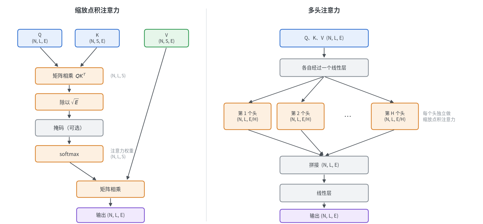
$Q$、$K$、$V$是同一个序列时称为自注意力,序列中每个位置都关注同一序列的所有位置;$Q$来自一个序列、$K$和$V$来自另一个序列时称为交叉注意力,解码器用它来读取编码器的输出
1
2
3
4
5
6
7
8
9
10
11
12
13
14
15
16
17
18
19
20
21
22
23
24
25
26
import math

import torch
import torch.nn.functional as F


def attention(query, key, value, mask=None):
    """mask中为True的位置不参与注意力"""
    scores = query @ key.transpose(-2, -1) / math.sqrt(query.size(-1))
    if mask is not None:
        scores = scores.masked_fill(mask, float("-inf"))
    weights = scores.softmax(dim=-1)
    return weights @ value, weights


query = torch.randn(2, 5, 64)  # (N, L, E)
key = torch.randn(2, 7, 64)    # (N, S, E)
value = torch.randn(2, 7, 64)  # (N, S, E)

out, weights = attention(query, key, value)
print(out.shape)            # torch.Size([2, 5, 64])
print(weights.shape)        # torch.Size([2, 5, 7])
print(weights.sum(dim=-1))  # 每一行的权重之和为1

# 与PyTorch自带的实现结果一致
print(torch.allclose(out, F.scaled_dot_product_attention(query, key, value), atol=1e-6))  # True
注意力权重的形状为$(N, L, S)$,需要的内存与序列长度的平方成正比,这是 Transformer 处理长序列时的主要瓶颈
多头注意力
多头注意力把$E$维的向量平均分成$H$份,每一份独立做一次注意力,最后再拼接起来。不同的头可以关注不同的关系,而总的计算量与单头基本相同
1
nn.MultiheadAttention(embed_dim, num_heads, dropout=0.0, bias=True, batch_first=False)
embed_dim必须能被num_heads整除,否则报错embed_dim must be divisible by num_heads- 前向传播的三个参数依次为
query、key、value,自注意力时传入同一个张量 - 返回值为输出和注意力权重,权重默认是各个头的平均
1
2
3
4
5
6
7
8
9
10
11
12
13
14
import torch
from torch import nn

x = torch.randn(2, 10, 64)
attention = nn.MultiheadAttention(embed_dim=64, num_heads=4, batch_first=True)

out, weights = attention(x, x, x)
print(weights.shape)  # torch.Size([2, 10, 10]),各个头的平均

out, weights = attention(x, x, x, average_attn_weights=False)
print(weights.shape)  # torch.Size([2, 4, 10, 10]),每个头各自的权重

out, weights = attention(x, x, x, need_weights=False)
print(weights)        # None,不需要权重时可以走更快的实现
掩码
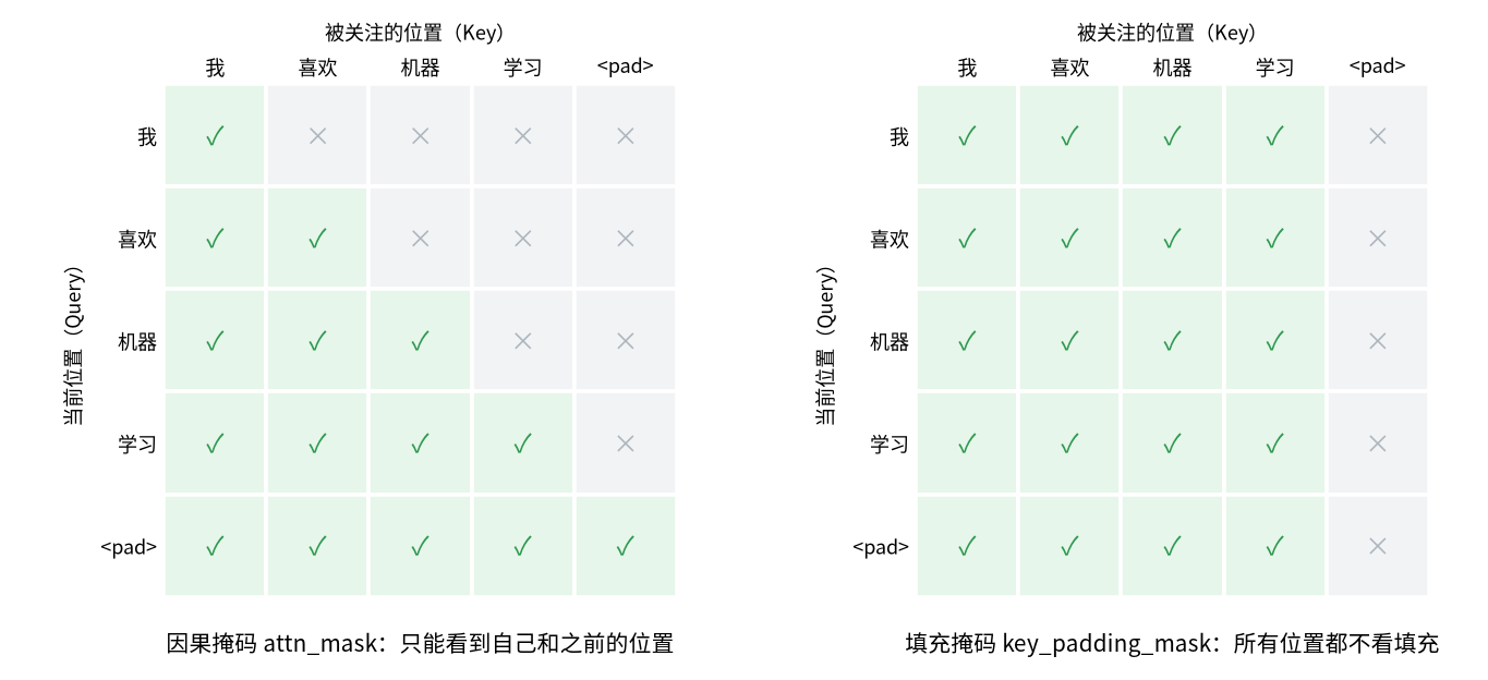
掩码用来禁止某些位置之间的注意力,有两种
| 参数 | 形状 | 作用 |
|---|---|---|
attn_mask | (L, S) | 指定每个位置可以关注哪些位置,最常见的是因果掩码,使每个位置只能看到自己和之前的位置 |
key_padding_mask | (N, S) | 标出每个序列中哪些位置是填充,所有位置都不再关注它们 |
一个批次中的句子长度不同,短的要用填充补齐,填充位置没有实际含义,需要用填充掩码屏蔽。语言模型在预测下一个词时不能看到后面的内容,需要用因果掩码
1
2
3
4
5
6
7
8
9
10
11
12
13
14
15
16
17
18
import torch
from torch import nn

torch.manual_seed(0)
x = torch.randn(1, 4, 8)
attention = nn.MultiheadAttention(embed_dim=8, num_heads=2, batch_first=True)

# 因果掩码:上三角为True,每个位置只能看到自己和之前的位置
causal_mask = torch.triu(torch.ones(4, 4, dtype=torch.bool), diagonal=1)
print(causal_mask)

_, weights = attention(x, x, x, attn_mask=causal_mask)
print(weights[0].round(decimals=2))  # 上三角全为0

# 填充掩码:最后一个位置是填充,所有位置都不关注它
padding_mask = torch.tensor([[False, False, False, True]])
_, weights = attention(x, x, x, key_padding_mask=padding_mask)
print(weights[0].round(decimals=2))  # 最后一列全为0
掩码有两种写法,含义不同:
| 类型 | 含义 |
|---|---|
| 布尔型 | True表示不允许关注 |
| 浮点型 | 直接加到相似度上,0表示允许,-inf表示不允许 |
nn.Transformer.generate_square_subsequent_mask(L)生成的是浮点型的因果掩码,与上面用torch.triu生成的布尔型掩码效果相同
F.scaled_dot_product_attention的布尔型掩码含义相反,True表示允许关注。 把同一个掩码从nn.MultiheadAttention搬到这个函数时需要取反
位置编码
注意力本身不区分顺序,把输入的词打乱,每个词得到的结果不变。因此需要在输入中加入位置信息,做法是给每个位置一个向量,与词向量相加
正弦位置编码
原始 Transformer 使用固定的正弦和余弦函数,不需要训练
\[PE_{(pos, 2i)} = \sin\left(\frac{pos}{10000^{2i/E}}\right) ,\qquad PE_{(pos, 2i+1)} = \cos\left(\frac{pos}{10000^{2i/E}}\right)\]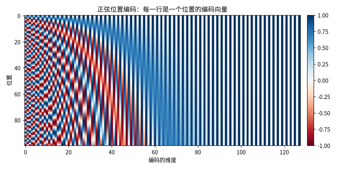
1
2
3
4
5
6
7
8
9
10
11
12
13
14
15
16
17
18
19
20
21
22
23
import math

import torch
from torch import nn


class PositionalEncoding(nn.Module):
    def __init__(self, d_model, max_len=5000):
        super().__init__()
        position = torch.arange(max_len).unsqueeze(1)
        div_term = torch.exp(torch.arange(0, d_model, 2) * (-math.log(10000.0) / d_model))

        pe = torch.zeros(max_len, d_model)
        pe[:, 0::2] = torch.sin(position * div_term)  # 偶数维用sin
        pe[:, 1::2] = torch.cos(position * div_term)  # 奇数维用cos
        self.register_buffer("pe", pe)                # 不参与训练,但随模型一起保存和移动

    def forward(self, x):
        return x + self.pe[: x.size(1)]  # x: (N, L, E)


x = torch.zeros(2, 10, 64)
print(PositionalEncoding(64)(x).shape)  # torch.Size([2, 10, 64])
可学习的位置编码
另一种做法是把位置编号当作词一样查表,用nn.Embedding(max_len, d_model)表示,随模型一起训练。BERT、GPT、ViT 都采用这种方式,实现更简单,缺点是无法处理比max_len更长的序列。下文的模型使用这种方式
旋转位置编码
前两种方式都是把位置向量加到输入上,表示的是绝对位置。旋转位置编码(RoPE)换了一种思路:不改动输入,而是在每次计算注意力时,把$Q$和$K$按各自所在的位置旋转一个角度。两个向量的点积只取决于它们的夹角,因此注意力的结果只与两个位置的相对距离有关,与绝对位置无关
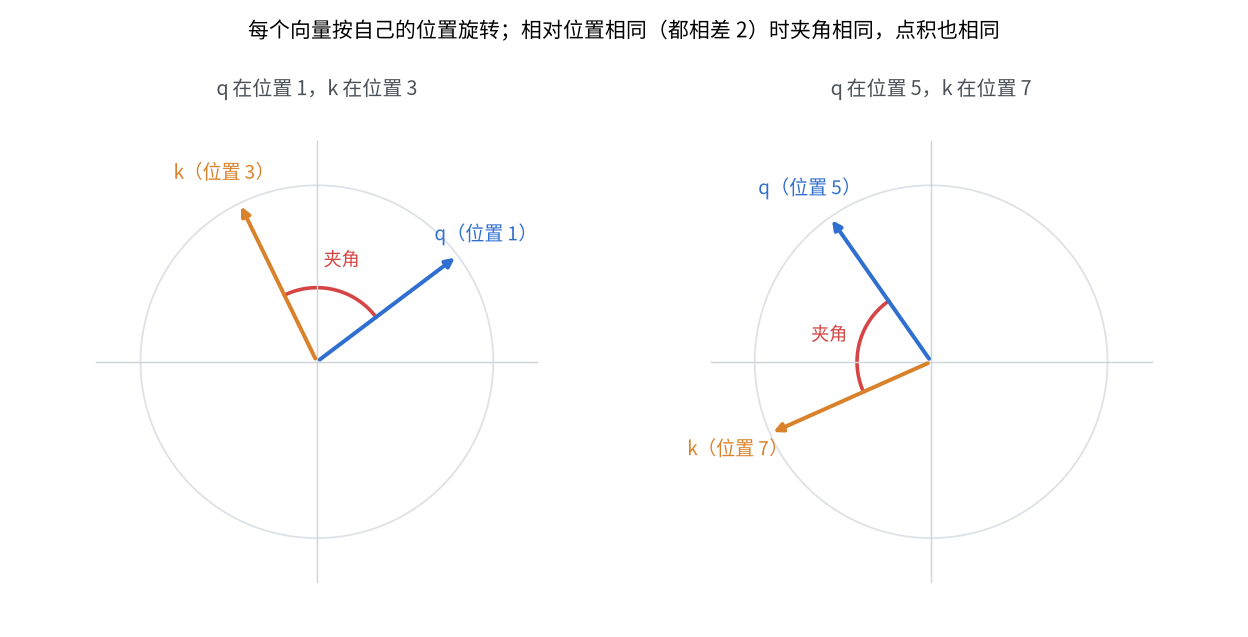
具体做法是把向量中相邻的两个维度看作一个二维向量,位置为$m$时旋转$m\theta$,不同的维度对使用不同的$\theta$,取值方式与正弦位置编码相同
1
2
3
4
5
6
7
8
9
10
11
12
13
14
15
16
17
18
19
20
21
22
23
24
25
26
27
28
29
30
31
import torch


def rope_angles(dim, length, base=10000.0):
    """返回每个位置、每对维度的旋转角度的cos和sin,形状均为(length, dim / 2)"""
    inv_freq = 1.0 / (base ** (torch.arange(0, dim, 2) / dim))
    angles = torch.outer(torch.arange(length), inv_freq)
    return angles.cos(), angles.sin()


def apply_rope(x, cos, sin):
    """x: (..., L, dim),把相邻的两个维度看作一个二维向量,按所在位置旋转"""
    x1, x2 = x[..., 0::2], x[..., 1::2]
    rotated = torch.stack([x1 * cos - x2 * sin, x1 * sin + x2 * cos], dim=-1)
    return rotated.flatten(-2)


torch.manual_seed(0)
cos, sin = rope_angles(dim=64, length=32)
q = torch.randn(64)
k = torch.randn(64)


def score(m, n):
    """q放在位置m、k放在位置n时的点积"""
    return (apply_rope(q, cos[m], sin[m]) * apply_rope(k, cos[n], sin[n])).sum()


print(torch.allclose(score(3, 1), score(10, 8), atol=1e-4))   # True,相对位置都是2
print(torch.allclose(score(3, 1), score(10, 5), atol=1e-4))   # False,相对位置不同
print(torch.allclose(apply_rope(q, cos[7], sin[7]).norm(), q.norm()))  # True,旋转不改变长度
- 只作用于注意力中的$Q$和$K$,不作用于$V$,也不加到输入上
- 没有需要训练的参数,也没有最大长度的限制
- 对相对位置敏感,在长序列上的效果通常好于可学习的位置编码,是目前大语言模型的主流做法
参数量计算
| 层 | 参数量 | 说明 |
|---|---|---|
nn.Embedding | 词表大小 × E | 词表很大时是模型中参数最多的部分 |
nn.MultiheadAttention | 4E² + 4E | Q、K、V 和输出各一个 E×E 的线性层,与头数无关 |
nn.LayerNorm | 2E | 每个维度一个缩放系数和一个偏移 |
| 前馈网络 | 2 × E × 中间维度 + 中间维度 + E | 两个线性层,中间维度通常取 4E |
| 位置编码 | 正弦为 0,可学习为最大长度 × E |
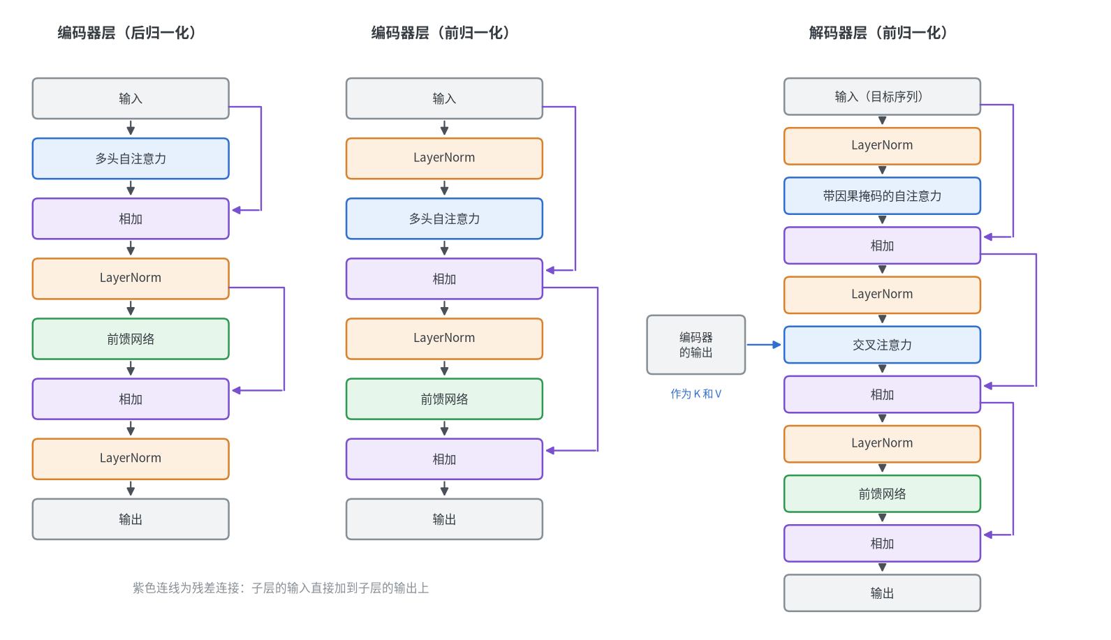
一个编码器层由一个多头注意力、一个前馈网络和两个LayerNorm组成;解码器层多一个交叉注意力和一个LayerNorm
1
2
3
4
5
6
7
8
9
10
11
12
13
from torch import nn


def count(module):
    return sum(p.numel() for p in module.parameters())


print(count(nn.Embedding(30000, 512)))                               # 15360000
print(count(nn.MultiheadAttention(512, 8)))                          # 1050624
print(count(nn.MultiheadAttention(512, 1)))                          # 1050624,与头数无关
print(count(nn.LayerNorm(512)))                                      # 1024
print(count(nn.TransformerEncoderLayer(512, 8, dim_feedforward=2048)))  # 3152384
print(count(nn.TransformerDecoderLayer(512, 8, dim_feedforward=2048)))  # 4204032
常用结构
| 结构 | 组成 | 常见于 |
|---|---|---|
| 编码器层 | 自注意力 + 前馈网络 | 所有 Transformer |
| 仅编码器模型 | 嵌入 + 多个编码器层 + 分类头 | BERT、文本分类、ViT |
| 仅解码器模型 | 嵌入 + 多个带因果掩码的编码器层 + 输出层 | GPT 等语言模型 |
| 编码器-解码器模型 | 编码器 + 带交叉注意力的解码器 | 翻译、摘要等序列到序列任务 |
编码器层
每个编码器层包含两个子层:多头自注意力和前馈网络,每个子层都带有残差连接和层归一化。归一化的位置有两种:
- 后归一化:先计算子层并相加,再归一化。原始 Transformer 的做法,层数多时训练不稳定
- 前归一化:先归一化,再计算子层并相加。现在更常用,训练更稳定
1
2
3
4
5
6
7
8
9
10
11
12
13
14
15
16
17
18
19
20
21
22
23
24
25
26
27
28
29
30
31
32
import torch
from torch import nn


class EncoderLayer(nn.Module):
    def __init__(self, d_model, num_heads, dim_feedforward, dropout=0.1):
        super().__init__()
        self.norm1 = nn.LayerNorm(d_model)
        self.attention = nn.MultiheadAttention(d_model, num_heads, dropout=dropout, batch_first=True)
        self.norm2 = nn.LayerNorm(d_model)
        self.feed_forward = nn.Sequential(
            nn.Linear(d_model, dim_feedforward),
            nn.GELU(),
            nn.Dropout(dropout),
            nn.Linear(dim_feedforward, d_model),
        )
        self.dropout = nn.Dropout(dropout)

    def forward(self, x, attn_mask=None, key_padding_mask=None):
        # 自注意力子层:先归一化,再计算,最后与输入相加
        y = self.norm1(x)
        y, _ = self.attention(y, y, y, attn_mask=attn_mask,
                              key_padding_mask=key_padding_mask, need_weights=False)
        x = x + self.dropout(y)

        # 前馈子层
        x = x + self.dropout(self.feed_forward(self.norm2(x)))
        return x


x = torch.randn(2, 10, 64)
print(EncoderLayer(64, 4, 256)(x).shape)  # torch.Size([2, 10, 64])
PyTorch 自带了相同的结构,norm_first=True为前归一化,默认为后归一化。nn.TransformerEncoder把同一个层复制多份堆叠起来
1
2
3
4
5
6
7
8
9
import torch
from torch import nn

layer = nn.TransformerEncoderLayer(d_model=64, nhead=4, dim_feedforward=256,
                                   batch_first=True, norm_first=True)
encoder = nn.TransformerEncoder(layer, num_layers=6, enable_nested_tensor=False)

x = torch.randn(2, 10, 64)
print(encoder(x).shape)  # torch.Size([2, 10, 64])
仅编码器模型
编码器的输出是每个位置一个向量,分类任务需要把它们合并为一个向量再接分类头。常见的合并方式是取平均,或者在序列开头加一个专门用于分类的[CLS]位置
1
2
3
4
5
6
7
8
9
10
11
12
13
14
15
16
17
18
19
20
21
22
23
24
25
26
27
28
29
30
31
import torch
from torch import nn


class TextClassifier(nn.Module):
    def __init__(self, vocab_size, num_classes, d_model=64, num_heads=4, num_layers=2, max_len=512):
        super().__init__()
        self.token_embedding = nn.Embedding(vocab_size, d_model, padding_idx=0)
        self.position_embedding = nn.Embedding(max_len, d_model)  # 可学习的位置编码
        layer = nn.TransformerEncoderLayer(d_model, num_heads, dim_feedforward=4 * d_model,
                                           batch_first=True, norm_first=True)
        self.encoder = nn.TransformerEncoder(layer, num_layers, enable_nested_tensor=False)
        self.norm = nn.LayerNorm(d_model)
        self.head = nn.Linear(d_model, num_classes)

    def forward(self, tokens):
        padding_mask = tokens == 0                                # (N, L),填充位置为True
        positions = torch.arange(tokens.size(1), device=tokens.device)
        x = self.token_embedding(tokens) + self.position_embedding(positions)
        x = self.norm(self.encoder(x, src_key_padding_mask=padding_mask))

        # 只对非填充位置取平均,得到整个句子的表示
        keep = (~padding_mask).unsqueeze(-1)                      # (N, L, 1)
        pooled = (x * keep).sum(dim=1) / keep.sum(dim=1)          # (N, E)
        return self.head(pooled)


tokens = torch.tensor([[5, 8, 2, 9, 0, 0],
                       [7, 3, 0, 0, 0, 0]])  # 0为填充
model = TextClassifier(vocab_size=1000, num_classes=3)
print(model(tokens).shape)  # torch.Size([2, 3])
padding_idx=0使编号为 0 的词向量恒为零并且不参与训练- 取平均时必须排除填充位置,否则同一句话补的填充越多,结果越被稀释
- 使用前归一化时,最后一个编码器层的输出没有经过归一化,需要在编码器之后再加一个
LayerNorm
图像块嵌入
ViT 把图像切成固定大小的小块,每一块作为序列中的一个位置,之后的结构与文本的编码器完全相同。切块和线性变换可以用一个卷积完成:卷积核大小和步幅都等于图像块的大小,$224 \times 224$的图像按$16 \times 16$切块,得到$14 \times 14 = 196$个位置
1
2
3
4
5
6
7
8
9
10
11
12
13
14
15
16
17
18
19
20
21
22
23
import torch
from torch import nn


class PatchEmbedding(nn.Module):
    def __init__(self, image_size=224, patch_size=16, in_channels=3, d_model=768):
        super().__init__()
        num_patches = (image_size // patch_size) ** 2
        # 卷积核大小与步幅都等于图像块大小,相当于对每个图像块做一次线性变换
        self.projection = nn.Conv2d(in_channels, d_model, kernel_size=patch_size, stride=patch_size)
        self.cls_token = nn.Parameter(torch.zeros(1, 1, d_model))
        self.position_embedding = nn.Parameter(torch.zeros(1, num_patches + 1, d_model))

    def forward(self, x):
        x = self.projection(x)            # (N, E, 14, 14)
        x = x.flatten(2).transpose(1, 2)  # (N, 196, E)
        cls_token = self.cls_token.expand(x.size(0), -1, -1)
        x = torch.cat([cls_token, x], dim=1)  # (N, 197, E)
        return x + self.position_embedding


x = torch.randn(2, 3, 224, 224)
print(PatchEmbedding()(x).shape)  # torch.Size([2, 197, 768])
仅解码器模型
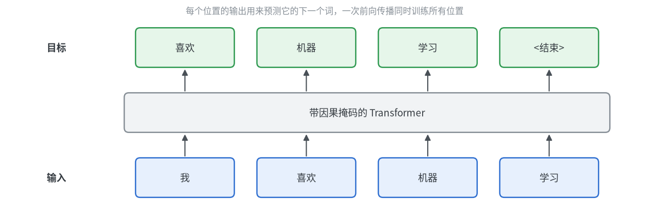
GPT 这类语言模型只有自注意力、没有交叉注意力,结构上就是加了因果掩码的编码器层,所以用nn.TransformerEncoder实现。每个位置的输出用来预测下一个词,因果掩码保证它看不到后面的内容
1
2
3
4
5
6
7
8
9
10
11
12
13
14
15
16
17
18
19
20
21
22
23
24
25
26
27
28
29
30
31
32
33
34
import torch
from torch import nn


class LanguageModel(nn.Module):
    def __init__(self, vocab_size, d_model=64, num_heads=4, num_layers=2, max_len=512):
        super().__init__()
        self.token_embedding = nn.Embedding(vocab_size, d_model)
        self.position_embedding = nn.Embedding(max_len, d_model)
        layer = nn.TransformerEncoderLayer(d_model, num_heads, dim_feedforward=4 * d_model,
                                           batch_first=True, norm_first=True)
        self.blocks = nn.TransformerEncoder(layer, num_layers, enable_nested_tensor=False)
        self.norm = nn.LayerNorm(d_model)
        self.head = nn.Linear(d_model, vocab_size)

    def forward(self, tokens):
        length = tokens.size(1)
        positions = torch.arange(length, device=tokens.device)
        causal_mask = torch.triu(torch.ones(length, length, dtype=torch.bool, device=tokens.device), diagonal=1)

        x = self.token_embedding(tokens) + self.position_embedding(positions)
        x = self.norm(self.blocks(x, mask=causal_mask))
        return self.head(x)  # (N, L, vocab_size),每个位置预测下一个词


model = LanguageModel(vocab_size=1000).eval()
tokens = torch.randint(0, 1000, (2, 10))
logits = model(tokens)
print(logits.shape)  # torch.Size([2, 10, 1000])

# 修改最后一个词,前面各位置的输出不变,说明没有看到后面的内容
changed = tokens.clone()
changed[:, -1] = (changed[:, -1] + 1) % 1000
print(torch.allclose(logits[:, :-1], model(changed)[:, :-1], atol=1e-5))  # True
编码器-解码器模型
翻译这类任务的输入和输出是两个不同的序列。编码器处理源序列,解码器在生成目标序列的每个位置时,通过交叉注意力读取编码器的输出。nn.Transformer包含了完整的编码器和解码器,但不包含嵌入、位置编码和输出层,需要自行添加
1
2
3
4
5
6
7
8
9
10
11
12
import torch
from torch import nn

model = nn.Transformer(d_model=64, nhead=4, num_encoder_layers=2, num_decoder_layers=2,
                       dim_feedforward=256, batch_first=True)

source = torch.randn(2, 12, 64)  # 源序列,已经过嵌入:(N, S, E)
target = torch.randn(2, 9, 64)   # 目标序列:(N, T, E)
target_mask = nn.Transformer.generate_square_subsequent_mask(9)

out = model(source, target, tgt_mask=target_mask)
print(out.shape)  # torch.Size([2, 9, 64])
训练时目标序列整体输入并加上因果掩码,一次得到所有位置的预测;推理时只能一个词一个词地生成,每次把已经生成的部分作为目标序列输入
语言模型的训练与生成
下面用一个完整的例子说明语言模型怎样训练、怎样逐词生成。以下代码按顺序放在同一个文件中,后面的部分会用到前面的定义
模型
这里没有使用nn.TransformerEncoder,而是手写了注意力层,因为后面的 KV 缓存需要控制注意力内部的计算。cache参数在训练时用不到,可以先忽略
1
2
3
4
5
6
7
8
9
10
11
12
13
14
15
16
17
18
19
20
21
22
23
24
25
26
27
28
29
30
31
32
33
34
35
36
37
38
39
40
41
42
43
44
45
46
47
48
49
50
51
52
53
54
55
56
57
58
59
60
61
62
63
64
65
66
67
68
69
import torch
import torch.nn.functional as F
from torch import nn


class CausalSelfAttention(nn.Module):
    def __init__(self, d_model, num_heads):
        super().__init__()
        self.num_heads = num_heads
        self.qkv = nn.Linear(d_model, 3 * d_model)
        self.proj = nn.Linear(d_model, d_model)

    def forward(self, x, cache=None):
        n, length, d_model = x.shape
        # (N, L, 3E) -> 3个(N, H, L, E / H)
        q, k, v = (self.qkv(x)
                   .view(n, length, 3, self.num_heads, d_model // self.num_heads)
                   .permute(2, 0, 3, 1, 4))

        past = 0
        if cache is not None:
            if "k" in cache:
                past = cache["k"].size(2)
                k = torch.cat([cache["k"], k], dim=2)  # 之前的K、V直接取缓存,只计算新位置的
                v = torch.cat([cache["v"], v], dim=2)
            cache["k"], cache["v"] = k, v

        # 新位置i可以关注缓存中的全部位置,以及新位置中不晚于自己的位置。True表示允许
        mask = torch.ones(length, past + length, dtype=torch.bool, device=x.device).tril(diagonal=past)
        out = F.scaled_dot_product_attention(q, k, v, attn_mask=mask)
        return self.proj(out.transpose(1, 2).reshape(n, length, d_model))


class Block(nn.Module):
    def __init__(self, d_model, num_heads):
        super().__init__()
        self.norm1 = nn.LayerNorm(d_model)
        self.attention = CausalSelfAttention(d_model, num_heads)
        self.norm2 = nn.LayerNorm(d_model)
        self.feed_forward = nn.Sequential(
            nn.Linear(d_model, 4 * d_model), nn.GELU(), nn.Linear(4 * d_model, d_model))

    def forward(self, x, cache=None):
        x = x + self.attention(self.norm1(x), cache)
        return x + self.feed_forward(self.norm2(x))


class GPT(nn.Module):
    def __init__(self, vocab_size, d_model=64, num_heads=4, num_layers=2, max_len=256):
        super().__init__()
        self.max_len = max_len
        self.token_embedding = nn.Embedding(vocab_size, d_model)
        self.position_embedding = nn.Embedding(max_len, d_model)
        self.blocks = nn.ModuleList(Block(d_model, num_heads) for _ in range(num_layers))
        self.norm = nn.LayerNorm(d_model)
        self.head = nn.Linear(d_model, vocab_size)

    def forward(self, tokens, caches=None):
        # 使用缓存时,输入的只是新的词,位置要从缓存的长度之后开始编号
        past = caches[0]["k"].size(2) if caches and "k" in caches[0] else 0
        positions = torch.arange(past, past + tokens.size(1), device=tokens.device)
        x = self.token_embedding(tokens) + self.position_embedding(positions)
        for i, block in enumerate(self.blocks):
            x = block(x, caches[i] if caches is not None else None)
        return self.head(self.norm(x))


model = GPT(vocab_size=1000)
print(model(torch.randint(0, 1000, (2, 10))).shape)  # torch.Size([2, 10, 1000])
训练循环
语言模型的训练目标是预测下一个词。把一段文本向后错开一个位置就得到目标:输入是第 1 到第 L 个词,目标是第 2 到第 L+1 个词。由于有因果掩码,每个位置只能看到自己和之前的词,所以一次前向传播可以同时训练所有位置
下面以字符为单位,在一句重复的文本上训练
1
2
3
4
5
6
7
8
9
10
11
12
13
14
15
16
17
18
19
20
21
22
23
24
25
26
27
text = "to be or not to be, that is the question. " * 50
chars = sorted(set(text))
encode = {ch: i for i, ch in enumerate(chars)}
data = torch.tensor([encode[ch] for ch in text])

torch.manual_seed(0)
model = GPT(vocab_size=len(chars))
optimizer = torch.optim.AdamW(model.parameters(), lr=3e-3, weight_decay=0.01)
batch_size, length = 32, 128

model.train()
for step in range(1, 301):
    # 随机截取若干段长度为length + 1的文本
    start = torch.randint(0, len(data) - length - 1, (batch_size,))
    batch = torch.stack([data[i:i + length + 1] for i in start])
    inputs, targets = batch[:, :-1], batch[:, 1:]  # 目标是输入向后错开一个位置

    logits = model(inputs)                         # (N, L, 词表大小)
    loss = F.cross_entropy(logits.reshape(-1, logits.size(-1)), targets.reshape(-1))

    optimizer.zero_grad()
    loss.backward()
    nn.utils.clip_grad_norm_(model.parameters(), max_norm=1.0)  # 梯度裁剪,防止个别批次的梯度过大
    optimizer.step()

    if step % 100 == 0:
        print(f"step {step}, loss {loss.item():.3f}")
1
2
3
step 100, loss 0.395
step 200, loss 0.019
step 300, loss 0.013
F.cross_entropy要求输入为 (样本数,类别数),所以把批大小和序列长度两个维度合并- 批次中有填充时,给
F.cross_entropy加上ignore_index参数,使填充位置不计入损失 - 训练前调用
model.train(),推理前调用model.eval(),两者的区别在于Dropout是否生效
逐词生成
训练时所有位置一次算完,生成时却只能一个词一个词地来:把已有的序列输入模型,取最后一个位置的输出作为下一个词的概率分布,从中选出一个词接到序列末尾,再重复这个过程
1
2
3
4
5
6
7
8
9
10
11
12
13
14
15
16
17
18
19
20
21
22
@torch.no_grad()
def generate(model, tokens, max_new_tokens, temperature=1.0, top_k=None):
    model.eval()
    for _ in range(max_new_tokens):
        logits = model(tokens[:, -model.max_len:])[:, -1]  # 只需要最后一个位置的输出
        if temperature == 0:
            next_token = logits.argmax(dim=-1, keepdim=True)  # 贪心:直接取概率最大的词
        else:
            logits = logits / temperature
            if top_k is not None:
                kth = logits.topk(top_k).values[:, [-1]]
                logits = logits.masked_fill(logits < kth, float("-inf"))  # 只保留概率最大的k个词
            next_token = torch.multinomial(logits.softmax(dim=-1), num_samples=1)
        tokens = torch.cat([tokens, next_token], dim=1)
    return tokens


decode = {i: ch for ch, i in encode.items()}
prompt = torch.tensor([[encode[ch] for ch in "to be"]])

out = generate(model, prompt, max_new_tokens=36, temperature=0)
print("".join(decode[i] for i in out[0].tolist()))
1
to be, that is the question. to be or not
| 参数 | 作用 |
|---|---|
temperature | 温度。为 0 时每次都取概率最大的词,结果固定;越大概率分布越平缓,结果越随机 |
top_k | 只在概率最大的 k 个词中采样,避免选到概率极低的词 |
使用可学习的位置编码时,生成的总长度不能超过训练时见过的长度,超出后位置向量没有经过训练,结果会变差
KV 缓存
上面的生成方式每生成一个词,都要把整个序列重新计算一遍,而其中绝大部分是重复的:由于因果掩码,前面位置的结果不受后面的词影响,每一步都完全相同
KV 缓存把每一层注意力中已经算过的$K$和$V$保存下来。之后每一步只输入新生成的那一个词,只计算它的$Q$、$K$、$V$,再与缓存中的$K$、$V$一起做注意力
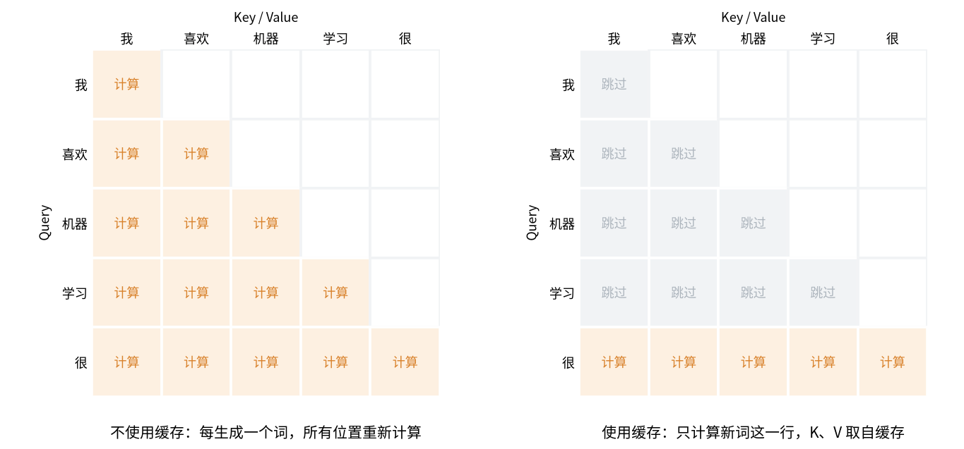
前面的CausalSelfAttention已经支持缓存:传入一个字典时,它会把新的$K$、$V$拼接到字典中已有的后面
1
2
3
4
5
6
7
8
9
10
11
12
13
14
15
16
17
18
19
20
21
22
23
24
25
import time


@torch.no_grad()
def generate_cached(model, tokens, max_new_tokens):
    model.eval()
    caches = [{} for _ in model.blocks]         # 每一层一份缓存
    logits = model(tokens, caches)[:, -1]       # 第一步:输入整个提示词,填满缓存
    for _ in range(max_new_tokens):
        next_token = logits.argmax(dim=-1, keepdim=True)
        tokens = torch.cat([tokens, next_token], dim=1)
        logits = model(next_token, caches)[:, -1]  # 之后每一步只输入新生成的一个词
    return tokens


start = time.perf_counter()
plain = generate(model, prompt, max_new_tokens=100, temperature=0)
plain_time = time.perf_counter() - start

start = time.perf_counter()
cached = generate_cached(model, prompt, max_new_tokens=100)
cached_time = time.perf_counter() - start

print(torch.equal(plain, cached))  # True,两种方式生成的结果完全相同
print(f"不使用缓存 {plain_time:.2f} 秒,使用缓存 {cached_time:.2f} 秒")
1
2
True
不使用缓存 0.02 秒,使用缓存 0.01 秒
- 两种方式的结果完全相同,缓存只是省去了重复计算
- 序列越长,节省得越多:不使用缓存时生成每个词的计算量与当前长度的平方成正比,使用缓存时只与长度成正比。这里的模型很小、序列很短,差距还不明显,耗时每次运行也会有波动。上面的耗时在 CPU 上测得,机器的配置为 Intel Core Ultra 9 285K、GeForce RTX 5090 D、64 GB 内存
- 代价是内存,每一层都要保存所有位置的$K$和$V$
- 使用缓存时,新词的位置编号要从缓存的长度之后开始,而不是从 0 开始
- 只适用于带因果掩码的模型;没有因果掩码时,新增一个词会改变所有位置的结果
较新的改进
原始 Transformer 之后,各个部分都出现了更常用的替代做法
| 部分 | 原始 Transformer | 现在常见的做法 |
|---|---|---|
| 归一化的位置 | 后归一化 | 前归一化,训练更稳定 |
| 归一化层 | LayerNorm | RMSNorm,只除以均方根,不减均值也没有偏移,参数减半 |
| 位置编码 | 正弦位置编码,加到输入上 | 旋转位置编码,在注意力中旋转 Q 和 K |
| 前馈网络 | 两个线性层加ReLU | 换成GELU,或使用带门控的 SwiGLU |
| 注意力的实现 | 显式算出权重矩阵 | F.scaled_dot_product_attention,自动选用更快、更省内存的实现 |
| 推理 | 每一步重新计算整个序列 | KV 缓存 |
| 输出层 | 独立的线性层 | 与词嵌入共享同一个权重矩阵,减少参数 |
1
2
3
4
5
6
7
8
9
10
11
12
13
14
15
16
17
18
19
20
21
22
23
24
25
import torch
import torch.nn.functional as F
from torch import nn


class SwiGLU(nn.Module):
    def __init__(self, d_model, hidden):
        super().__init__()
        self.gate = nn.Linear(d_model, hidden, bias=False)
        self.up = nn.Linear(d_model, hidden, bias=False)
        self.down = nn.Linear(hidden, d_model, bias=False)

    def forward(self, x):
        return self.down(F.silu(self.gate(x)) * self.up(x))


x = torch.randn(2, 10, 64)
print(nn.RMSNorm(64)(x).shape)   # torch.Size([2, 10, 64])
print(SwiGLU(64, 170)(x).shape)  # torch.Size([2, 10, 64])

# 权重共享:输出层与词嵌入使用同一个矩阵
embedding = nn.Embedding(30000, 512)
head = nn.Linear(512, 30000, bias=False)
head.weight = embedding.weight
print(head.weight is embedding.weight)  # True
- SwiGLU 有三个线性层,中间维度通常取原来的三分之二,使参数量与普通的前馈网络大致相同
- 权重共享要求词嵌入和输出层的形状互为转置,输出层不能带偏置
查看各层的输出形状
torchinfo同样适用于 Transformer。输入是整数编号时不能用input_size,要用input_data传入一个实际的张量。以上面的文本分类模型为例
1
2
3
4
5
from torchinfo import summary

model = TextClassifier(vocab_size=1000, num_classes=3)
tokens = torch.randint(1, 1000, (2, 16))
summary(model, input_data=tokens, depth=2)
1
2
3
4
5
6
7
8
9
10
11
12
13
14
15
===============================================================================================
Layer (type:depth-idx)                        Output Shape              Param #
===============================================================================================
TextClassifier                                [2, 3]                    --
├─Embedding: 1-1                              [2, 16, 64]               64,000
├─Embedding: 1-2                              [16, 64]                  32,768
├─TransformerEncoder: 1-3                     [2, 16, 64]               --
│    └─ModuleList: 2-1                        --                        99,968
├─LayerNorm: 1-4                              [2, 16, 64]               128
├─Linear: 1-5                                 [2, 3]                    195
===============================================================================================
Total params: 197,059
Trainable params: 197,059
Non-trainable params: 0
===============================================================================================